# Introduction
Monitor what matters, find what is broken, and fix it.
## What is NannyML Cloud?
NannyML Cloud is a machine learning monitoring platform to monitor, analyze, and improve ML models in production.
To monitor today’s and tomorrow’s ML models properly, we need solutions that frame the monitoring problem better, solutions that have full coverage, and that monitor the model, not just its features. Because of this, NannyML Cloud focuses on model performance estimation and takes a performance-centric monitoring approach. Our monitoring approach goes as follows.
## The NannyML way
### 1. Monitor what matters
Focus on one single metric to know how your model is performing and get alerted when the performance drops.
* **Estimate model performance:** Know the performance of your ML models 24/7. NannyML estimates the performance of your ML models even if the ground truth is delayed or absent.
* **Measure the business impact of your models:** Tie the performance of your model to monetary or business-oriented outcomes. So that you always know what your ML brings to the table.
* **Avoid alert fatigue:** Traditional ML monitoring tends to overwhelm teams with many false alarms. By focusing on what matters, NannyML alerts are always meaningful.
Estimated Accuracy using Probabilistic Adaptive Performance Estimation (PAPE)
### 2. Find what is broken
If something is broken, understand the underlying causes by correlating performance issues with data drift alerts and concept drift variations. This approach provides an actionable path for solving model performance issues.
* **Measure the impact of Concept Drift** **on model performance:** Our concept drift algorithms use the latest ground-truth data to validate if the performance change has been due to a change of concept.
* **Uncover the most subtle changes in the data structure:** Leverage our multivariate drift detection method to uncover changes that univariate approaches cannot detect.
* **Go on a granular investigation:** Apply univariate drift detection methods allow to perform a granular investigation across the model's features. And easily find which ones correlate with the performance changes.
* **Intelligent alert ranking:** NannyML links back data drift alerts to changes in the model performance. So you can easily detect which features are causing the performance issues.
* **Segment your data for better interpretability:** Use segmentation to divide a dataset into meaningful subgroups, allowing you to monitor and analyze specific subsets of the population more effectively.
Concept drift detection panel
### 3. Fix it
Once you understand what went wrong, it becomes possible to tell whether a model is worth retraining, refactoring or if another issue resolution strategy is needed.
* **Retrain only when necessary:** Leverage [NannyML Cloud SDK](https://github.com/NannyML/docs/blob/v0.22.0/broken-reference/README.md) to automate monitoring data ingestion and the [webhooks](/cloud/deployment/application-setup/webhooks) to trigger retraining pipelines when the estimated performance drops.
## How to set up NannyML Cloud?
NannyML Cloud is available on both the Azure and AWS marketplaces, and you can deploy it in two different ways, depending on your needs.
* **Managed Application:** With the Managed application, no data will leave your environment. This option will provision the NannyML Cloud components and the required infrastructure within your Azure or AWS subscription. To learn more about this, check out the docs on how to set up NannyML Cloud on [Azure](/cloud/deployment/azure/azure-managed-application) and [AWS](/cloud/deployment/aws).
* **Software-as-a-Service (SaaS):** With the SaaS option, you send us the monitoring data, and the monitoring happens in our infrastructure. To learn more about this, check out the docs on how to set up NannyML Cloud on [Azure](/cloud/deployment/azure/azure-software-as-a-service-saas) and [AWS](/cloud/deployment/aws).
## NannyML OSS vs NannyML Cloud
NannyML Cloud, built on our open-source [NannyML library](https://github.com/nannyml/nannyml), adds new features and algorithms into an all-in-one monitoring platform.
Feature
NannyML OSS
NannyML Cloud
Performance estimation - CBPE and DLE
✅
✅
PAPE - 10% better performance estimations than CBPE
❌
✅
Concept shift detection
❌
✅
Covariate shift detection
✅
✅
Data quality checks
✅
✅
Intelligent alerting
✅
✅
Interactive visualizations
✅
✅
Slack and email notifications
❌
✅
Customizable dashboards
❌
✅
Programmatic data collection
❌
✅
Metric storage
❌
✅
Scheduling monitoring runs
❌
✅
Segmentation
❌
✅
Feature
NannyML OSS
NannyML Cloud
Performance estimation - CBPE and DLE
✅
✅
PAPE - 10% better performance estimations than CBPE
❌
✅
Concept shift detection
❌
✅
Covariate shift detection
✅
✅
Data quality checks
✅
✅
Intelligent alerting
✅
✅
Interactive visualizations
✅
✅
Slack and email notifications
❌
✅
Customizable dashboards
❌
✅
Programmatic data collection
❌
✅
Metric storage
❌
✅
Scheduling monitoring runs
❌
✅
Segmentation
❌
✅
## Where to go next?
Here, you can find several helpful guides to aid with onboarding.
Learn how the NannyML Cloud model monitoring works under the hood
# Quickstart
Get familiar with NannyML Cloud by monitoring a hotel booking cancellation prediction model.
## Getting access
If you don't have access yet, NannyML Cloud is available on both the Azure and AWS marketplaces, and you can deploy it in two different ways, depending on your needs.
* **Managed Application:** With the Managed application, no data will leave your environment. This option will provision the NannyML Cloud components and the required infrastructure within your own Azure or AWS subscription. To learn more about this, check out the docs on how to set up NannyML Cloud on [Azure](/cloud/deployment/azure/azure-managed-application) and [AWS](/cloud/deployment/aws).
* **Software-as-a-Service (SaaS):** With the SaaS option, you send us the monitoring data, and the monitoring happens in our own infrastructure. To learn more about this, check out the docs on how to set up NannyML Cloud on [Azure](/cloud/deployment/azure/azure-software-as-a-service-saas) and [AWS](/cloud/deployment/aws).
## Monitoring a classification model
If you prefer a video walkthrough, here's our Quickstart YouTube guide:
{% embed url="" %}
### Hotel booking prediction model
The dataset comes from two hotels in Portugal and has 30 features describing the booking entry. To learn more about this data, check out the [hotel booking demand dataset](https://www.sciencedirect.com/science/article/pii/S2352340918315191). After simple preprocessing, we trained the model to predict whether the booking would be canceled or not, with the final result of 0.87 ROC AUC on a test set.
To monitor the model in production, we created reference and analysis sets. NannyML uses the reference set to establish a baseline for model performance and shift detection. The test set is an ideal candidate to serve as a reference. The analysis set is the production data - NannyML checks if the model maintains performance or if there's a concept or covariate shift.
{% hint style="info" %}
Note that analysis data is sometimes referred to as monitored data.
{% endhint %}
Let's add our model:
{% tabs %}
{% tab title="NannyML Cloud UI" %}
1. Click on the **Add New Model** button in the navigation bar.
2. Complete the new model setup configuration.
New model configuration setup.
3. Upload the reference dataset by choosing one of the available upload methods (see image below). For this example, we will use the following links:
1. **Reference dataset link -** `https://raw.githubusercontent.com/NannyML/sample_datasets/main/hotel_booking_dataset/hotel_booking_reference_march.csv`
2. **Analysis dataset link** - `https://raw.githubusercontent.com/NannyML/sample_datasets/main/hotel_booking_dataset/hotel_booking_analysis_march.csv`
Data upload options
4. Configure the reference dataset. The uploaded reference data contains the following:
1. **Timestamp** - the information when the booking was made. The reference data spans from May to September 2016, while the analysis data covers October 2016 to August 2017.
2. **Identifier** - a unique identifier for each row in the dataset.
3. **Target** - ground truth/labels. In this example, the target is whether a booking is canceled or not. Notice that the target is not available in the analysis set. In this way, we simulate a real-world scenario where the ground truth is only available after some time.
4. **Predictions** - the predicted class. Whether the booking will get canceled or not
5. **Predicted probability** - the model scores outputted by the model.
6. **Model inputs** - 27 features about hotel booking, including booking like customer's country of origin, age, children, etc.
Optionally indicate the columns you wish to use for segmentation. This can be done by selecting specific columns using the **Segment by** dropdown menu or by selecting the **Segment by** flag for specific columns.
Reference dataset setup
5. Upload the analysis data in the same way you uploaded the reference dataset.
6. Next, upload the target data if it is available (in our working example, we don't have access to target data).
Upload target data if available
7. Configure the metrics you wish to evaluate.
Metrics
8. Finally, review and upload the model.
{% endtab %}
{% tab title="NannyML Cloud SDK" %}
To get started, simply follow the initial steps outlined in the [SDK documentation](/cloud/nannyml-cloud-sdk/getting-started). This will guide you through installing the SDK library and obtaining the NannyML Cloud URL and API Token.
After successful installation, create a Python script, import the SDK and Pandas library, and add the credentials.
{% hint style="info" %}
For demonstration purposes, we recommend using a Jupyter or Colab notebook to upload data with the SDK instead of a Python script.
{% endhint %}
```python
import pandas as pd
import nannyml_cloud_sdk as nml_sdk
nml_sdk.url = "your instance URL goes here eg; https://beta.app.nannyml.com"
nml_sdk.api_token = r"api token goes here"
```
Now, we will load reference and analysis data.
```python
reference_data = pd.read_csv("https://raw.githubusercontent.com/NannyML/sample_datasets/main/hotel_booking_dataset/hotel_booking_reference.csv")
analysis_data = pd.read_csv("https://raw.githubusercontent.com/NannyML/sample_datasets/main/hotel_booking_dataset/hotel_booking_analysis_march.csv")
```
We can now use the [Schema](https://nannyml.github.io/nannyml-cloud-sdk/api_reference/model/) class together with the `from_df()` method to configure the schema of the model.
```python
schema = nml_sdk.Schema.from_df(
'BINARY_CLASSIFICATION',
reference_data,
target_column_name='is_canceled',
identifier_column_name = 'Index',
)
```
Then, we create a new model by using the `Model.create()` method. Where we can set chunk period to monthly, and accuracy as the main monitoring performance metric.
```python
model = nml_sdk.Model.create(
name='Hotel Booking SDK upload',
schema=schema,
chunk_period='MONTHLY',
reference_data=reference_data,
analysis_data=analysis_data,
target_data=pd.DataFrame(columns=["Index", "is_canceled"]),
main_performance_metric='ACCURACY',
)
```
And voila, the model should now be available in your Model Overview dashboard! 🚀
{% endtab %}
{% endtabs %}
## Estimated performance
ML models are deployed to production once their performance has been validated and tested. This usually takes place in the model development phase. The main goal of ML model monitoring is to continuously verify whether the model maintains its anticipated performance (which is not the case most of the time).
Monitoring performance is relatively straightforward when targets are available, but in many use cases like demand forecasting or insurance pricing, the labels are delayed, costly, or impossible to get. In such scenarios, estimating performance is the only way to verify if the model is still working properly.
Let's see the estimated performance of our model on the summary page. The model summary shows signs of performance degradation in the last chunks of performance estimation.
The accuracy plot in the model summary page.
Also, the PCA reconstruction error from the multivariate drift detection method seems to be higher than the given thresholds.
The PCA reconstruction error plot in the model summary page.
{% hint style="info" %}
Notice that concept shift detection is not available since it requires ground truth data in the analysis set.
{% endhint %}
Multivariate drift detection is the first step in covariate shift detection, focusing on detecting any changes in the data structure over time. The accuracy and reconstruction error plot shows alerts in the last three months, which tells us that covariate shift is possibly responsible for it. But we still don't know what real-world changes are causing this. To figure that out, we need to analyze the drifting features more deeply.
## Why did the performance drop?
Once we’ve identified a performance issue, we need to troubleshoot it. The first step is to look into potential distribution shifts for all the features in the covariate shift panel.
We have six methods to determine the amount of shift in each feature. To begin the process, we focus on the four most important features: **hotel**, **lead\_time**, **parking\_spaces**, and **country**. These features were determined using the feature importance method after the model was trained. To streamline the analysis, the methods used are **l-infinity** for categorical variables and the **Wasserstein** method for continuous features.
L-infinity plot for country feature.
L-infinity plot for hotel feature.
Wasserstein distance plot for lead_time feature.
Wasserstein distance plot for parking_spaces feature.
For the features **country** and **hotel**, we noticed a shift in February that lines up with a drop in performance. Also, **lead\_time** began to drift from December to March, which is exactly when we started seeing a gradual decline in accuracy. So, it looks like the root cause is linked to the drift in these three features. Now, let's reason more broadly about these shifts and relate them to the customer's behavior around that time.
## Shift explanations
The root cause is associated with the drift in three key features: **lead\_time**, **hotel**, and **country**. During November-March, it's common for the temperatures in northern European countries like Germany, Sweden, and the Netherlands to drop below 0 degrees. Additionally, many children had their winter break at that time, allowing them to travel with their parents. It's possible that tourists from northern Europe chose to visit Portugal during this period to escape the cold, which explains the shift in the country's feature distribution.
Furthermore, Portugal's sunny weather and temperatures around 20 degrees are mainly found in Algarve, the southern part of the country, as opposed to Lisbon, where temperatures are around 15 degrees. This accounts for the shift in the hotel distribution feature, as more people are booking hotels in the Algarve. Lastly, many of these winter getaways by foreigners are typically planned well in advance to secure travel tickets, make train reservations, request time off from work, and make other preparations. This advanced planning explains the significant shift in the lead time feature.
These changes ultimately resulted in a decrease in the performance of the model during the December to March period.
## Comparing estimated and realized performance
We used performance estimation before since our analysis set didn't have targets. Now, we can add to validate the estimations and see if the concept drift has also affected the performance.
{% tabs %}
{% tab title="NannyML Cloud UI" %}
1. Go to [Model settings](/cloud/product-tour/model-side-panel/model-settings).
2. Click on the **Add new rows** button.
Datasets section in Model settings.
3. Upload the target dataset via the following link: - `https://raw.githubusercontent.com/NannyML/sample_datasets/main/hotel_booking_dataset/hotel_booking_gt_march.csv`
4. Run the analysis.
{% endtab %}
{% tab title="NannyML Cloud SDK" %}
We first need to load our target data before we upload it to the NannyML Cloud. Once we've done that, just run NannyML Cloud again to view the realized performance and concept shift results.
```python
target_data = pd.read_csv("https://raw.githubusercontent.com/NannyML/sample_datasets/main/hotel_booking_dataset/hotel_booking_gt_march.csv")
model_id = model["id"]
nml_sdk.Model.add_analysis_target_data(model_id, target_data)
nml_sdk.Run.trigger(model_id)
```
{% endtab %}
{% endtabs %}
The performance dashboard with a comparison plot between realized and estimated performance.
We can see that the realized performance also dropped in December, January, and February, confirming that the estimations were really accurate. Let's check if the concept drift is present in our data.
## Concept drift detection
The concept drift dashboard with a plot showing the impact of concept drift on accuracy.
The graph illustrates the impact of concept drift on performance, with the x-axis representing the change in accuracy due to concept drift. As we can see, it's less than -0.01 and remains within the specified thresholds, not triggering any alerts. This suggests that concept drift did not contribute to a drop in accuracy during that period, only previously analyzed covariate shift!
## What's next?
# Data Preparation
How to prepare your data before using NannyML
What data does NannyML need to monitor a machine learning model in production?
* Data from 2 different data periods are needed.
* Data needs to be in tabular format.
* Features, model outputs, and target (targets are optional for the monitored dataset).
* Some additional columns needed, namely a timestamp and an identifier column.
The NannyML open-source library provides sample datasets. Let's have a quick preview of the [synthetic car loan dataset](https://nannyml.readthedocs.io/en/stable/datasets/binary_car_loan.html) before we go into details.
```python
import nannyml as nml
reference, monitored, targets = nml.load_synthetic_car_loan_dataset()
reference.head()
```
id
timestamp
car_value
salary_range
debt_to_income_ratio
loan_length
repaid_loan_on_prev_car
size_of_downpayment
driver_tenure
repaid
y_pred_proba
y_pred
0
2018-01-01 00:00:00.000
39811
40K - 60K €
0.63295
19
False
40%
0.212653
1
0.99
1
1
2018-01-01 00:08:43.152
12679
40K - 60K €
0.718627
7
True
10%
4.92755
0
0.07
0
2
2018-01-01 00:17:26.304
19847
40K - 60K €
0.721724
17
False
0%
0.520817
1
1
1
3
2018-01-01 00:26:09.456
22652
20K - 20K €
0.705992
16
False
10%
0.453649
1
0.98
1
4
2018-01-01 00:34:52.608
21268
60K+ €
0.671888
21
True
30%
5.69526
1
0.99
1
Let's now see the requirements in more detail.
### Datasets and Periods
In order to monitor a model's behavior, we first need to establish a pattern of acceptable behavior. This is done by data from a reference period, often called **reference dataset**. Usually, this dataset is the test set from when the model was developed, or the latest available production data were the model performed according to expectations.
Then we need a **monitored dataset**, which is a dataset that comes from the period where we want to examine how well a model performs.
In some cases, the monitored datasets does not contain targets. This often happens when targets are available at a date later than when the prediction is made. To accommodate for this NannyML allows for a third dataset, the **target dataset.** The target dataset only needs to contain targets and an identifier column.
Also note that the same column names must be used in the reference, monitored and target datasets.
### Data Format
As can be seen in the above example NannyML consumes data in a tabular format. Each prediction is expected to be described in one row. Features and other information are provided through columns. An example can be seen in the sample data presented above. NannyML accepts data in csv and parquet formats.
### Features, Model Outputs and Targets
Those are the key information needed to monitor a model. All the features and model outputs are expected to be represented by unique columns in the data provided. By outputs we mean both predicted probabilities and predicted classes for classification problems. For the reference dataset model targets are required. For the monitored data they are optional. If they are not provided they can be added later through the target dataset option. Unless this is done, NannyML features such as realized performance and concept drift monitoring cannot be used.
### Additional Columns
Apart from the standard features NannyML needs two additional columns, an **id** column and a **timestamp** column.
#### Id column
An id column is a column that provides a unique identifier for each model prediction. Since each prediction is expected to be in one row the id column is unique per row in our data. It can be integer or a string. If a unique identifier is not present in your data, you need to create one before you can use NannyML Cloud.
#### Timestamp Column
The timestamp column is a column that describes the time at which a model prediction was made. It is mainly used in order to aggregate predictions according to when they were made in order to organize model monitoring results.
If that information is not stored for your business use case, you need to create a synthetic timestamp column before using NannyML. Note that timestamp information is used in [chunking](https://nannyml.readthedocs.io/en/stable/tutorials/chunking.html) and when plotting results so be careful to use values that will make sense. Any format supported by pandas can be used.
## Data Preparation Workflow
Given all of the above, how would one go about creating datasets to monitor their model with NannyML Cloud? Let's list the necessary steps:
1. Decide on which data period will be used for the reference dataset and which for the monitored dataset.
2. Gather relevant data from where they are stored.
1. Identify what data need to be collected. They are features, model outputs, targets as well as an id and a timestamp column.
2. Create queries to gather relevant data. This can be complicated if data are stored in different places. Keep in mind that the end results need to be data in tabular format.
3. Add required additional columns if they are not present.
4. Store the data. Note that NannyML can receive data from:
1. A public URL serving the raw file.
2. A cloud storage option, namely S3 and Azure blob storage.
3. Local files in your computer if their size is less than 100Mb.
4. The NannyML Cloud SDK.
Hence store the data in a way that is most convenient for you.
{% hint style="info" %}
We recommend storing your data as parquet files.
NannyML Cloud supports both parquet and CSV files, but CSV files don't store data type information. CSV files may cause incorrect data types to be inferred. If you later add more data to the model using the SDK or using parquet format, a data type conflict may occur.
{% endhint %}
# How to get data ready for NannyML
This tutorial is a practical guide on how to get your data in the right format to monitor your models with NannyML. We will illustrate step-by-step how to prepare data for monitoring. We will start with building a simple model that we will monitor later.
## Step 1: Have a trained model (prerequisite)
If you are looking into monitoring, you probably already have a model, a training set, and most likely some production (monitored) data on which you would like to check how your model is doing. This tutorial uses the [Banana Quality Prediction](https://github.com/NannyML/sample_datasets/tree/main/banana_quality) dataset to illustrate how to prepare your data.
Let's start by partitioning our data into three sets:
* Training
* Testing
* Monitored (production data)
{% hint style="info" %}
In a real scenario, you won't need to create the monitoring partition since this will naturally come after deploying the model.
If you already have a trained model, skip to [Step 2: Building a reference dataset.](#step-2-building-a-reference-dataset)
{% endhint %}
```python
import pandas as pd
url = 'https://raw.githubusercontent.com/NannyML/sample_datasets/main/banana_quality/banana_quality.csv'
data = pd.read_csv(url)
train_df, test_df, monitor_df = data.iloc[0:4000], data.iloc[4000:6000], data.iloc[6000:8000]
```
```python
data.head()
```
| Identifier | Timestamp | Size | Weight | Sweetness | Softness | HarvestTime | Ripeness | Acidity | Quality |
| ---------- | ------------------- | --------- | --------- | --------- | --------- | ----------- | --------- | --------- | ------- |
| 0 | 2020-01-01 00:00:00 | 2.622631 | -1.531197 | -0.293286 | 2.086239 | 4.379607 | 0.865033 | 0.139479 | 1 |
| 1 | 2020-01-01 00:30:00 | -3.592020 | 0.220773 | 0.298705 | -1.759699 | -4.116195 | 0.604932 | -2.387580 | 1 |
| 2 | 2020-01-01 01:00:00 | 1.270482 | -3.959625 | -3.447087 | 0.799014 | 0.148791 | -2.098769 | 0.727079 | 0 |
| 3 | 2020-01-01 01:30:00 | -0.002022 | -1.417225 | -1.847301 | 0.301628 | 1.364337 | 0.265501 | -0.458392 | 1 |
| 4 | 2020-01-01 02:00:00 | -0.786569 | -4.323583 | 1.466369 | 0.157923 | -2.063598 | 2.619294 | -0.340423 | 0 |
The **Quality** column is the target variable. It is encoded as:
* **1** - Good banana quality
* **0** - Bad banana quality
Once we have the data separated, we can build a simple model.
```python
from lightgbm import LGBMClassifier
features = [
'Size', 'Weight', 'Sweetness', 'Softness',
'HarvestTime', 'Ripeness', 'Acidity'
]
target = 'Quality'
timestamp = 'Timestamp'
clf = LGBMClassifier()
clf.fit(train_df[features], train_df[target])
```
Let's quickly check its performance on the training and testing sets before moving to the next step.
```python
from sklearn.metrics import roc_auc_score
roc_auc_train = roc_auc_score(
train_df[target], clf.predict_proba(train_df[features])[:, 1]
)
roc_auc_test = roc_auc_score(
test_df[target], clf.predict_proba(test_df[features])[:, 1]
)
print(f"ROC-AUC (train): {roc_auc_train}")
print(f"ROC-AUC (test): {roc_auc_test}")
```
```
ROC-AUC (train): 1.0
ROC-AUC (test): 0.9931109775641026
```
Looks like the model is doing a nice job in the training and testing datasets.
## Step 2: Building a reference dataset
Once we have a model that performs well on the test set, we can use it to build a reference dataset.
**Reference dataset:** The reference dataset is a benchmark set where the model behaves as expected. It is important that this dataset was not seen by the model during training. It should include targets and the model's predictions. In this tutorial, we will use the test set to build the reference set.
NannyML uses the reference dataset to establish a baseline of how the monitoring data and the model predictions should look after deployment. Internally, it uses it to calibrate most of its performance estimation methods and calculate the default threshold values for every monitored metric.
To transform the test dataset into a reference dataset, all we need to do is add the predicted probabilities and the model predictions to the test dataset.
This means that we will create the following columns:
* **y\_pred\_proba**: contains the model's predicted probabilities (scores) for class 1 (Good quality banana, in this case).
* **y\_pred**: contains the model's predicted class (0 or 1).
```python
reference_df = test_df.copy()
reference_df['y_pred_proba'] = clf.predict_proba(test_df[features])[:, 1]
reference_df['y_pred'] = clf.predict(test_df[features])
```
```python
reference_df.head()
```
| Identifier | Timestamp | Size | Weight | Sweetness | Softness | HarvestTime | Ripeness | Acidity | Quality | y\_pred\_proba | y\_pred |
| ---------- | ------------------- | --------- | --------- | --------- | --------- | ----------- | --------- | --------- | ------- | -------------- | ------- |
| 4000 | 2020-03-24 08:00:00 | -1.005942 | 0.457455 | -0.819113 | 1.014088 | 1.380156 | -2.005996 | 3.522873 | 0 | 0.002104 | 0 |
| 4001 | 2020-03-24 08:30:00 | -2.425685 | 1.682808 | -2.041250 | -1.925259 | -1.118302 | -1.264770 | -3.848056 | 0 | 0.006822 | 0 |
| 4002 | 2020-03-24 09:00:00 | 0.363760 | -1.777900 | -0.585864 | 2.736269 | 3.509048 | 1.986182 | -1.747902 | 1 | 0.998873 | 1 |
| 4003 | 2020-03-24 09:30:00 | -2.206337 | -3.712593 | 0.734068 | -2.015895 | -3.488548 | 0.747031 | 0.754206 | 0 | 0.019571 | 0 |
| 4004 | 2020-03-24 10:00:00 | 0.649706 | -3.580519 | 0.352195 | 1.058788 | 0.834113 | 3.243598 | -3.792337 | 1 | 0.967419 | 1 |
{% hint style="info" %}
We recommend storing your data as parquet files.
NannyML Cloud supports both parquet and CSV files, but CSV files don't store data type information. CSV files may cause incorrect data types to be inferred. If you later add more data to the model using the SDK or using parquet format, a data type conflict may occur.
{% endhint %}
## Step 3: Setting up the monitored dataset
**Monitored dataset:** This is the data that NannyML will monitor. It typically contains the latest production data, which should be after the reference period ends. This dataset does not require targets.
Similarly, as with the reference dataset, let's add the following columns to the monitored dataset.
* **y\_pred\_proba**: contains the model's predicted probabilities (scores) for class 1 (Good quality banana, in this case).
* **y\_pred**: contains the model's predicted class (0 or 1).
```python
monitor_df['y_pred_proba'] = clf.predict_proba(monitor_df[features])[:, 1]
monitor_df['y_pred'] = clf.predict(monitor_df[features])
```
```python
monitor_df.head()
```
| Identifier | Timestamp | Size | Weight | Sweetness | Softness | HarvestTime | Ripeness | Acidity | Quality | y\_pred\_proba | y\_pred |
| ---------- | ------------------- | --------- | --------- | --------- | --------- | ----------- | --------- | --------- | ------- | -------------- | ------- |
| 6000 | 2020-05-05 00:00:00 | -1.955202 | -0.117761 | 0.121855 | -5.150094 | -1.387223 | 3.435446 | 1.662624 | 1 | 0.999419 | 1 |
| 6001 | 2020-05-05 00:30:00 | -0.940370 | -1.119835 | -0.998754 | 1.206442 | -3.871381 | 0.711751 | 0.799148 | 0 | 0.001309 | 0 |
| 6002 | 2020-05-05 01:00:00 | -0.819169 | -3.060052 | -1.092720 | 2.581883 | -0.306439 | -2.864940 | -1.350002 | 0 | 0.000332 | 0 |
| 6003 | 2020-05-05 01:30:00 | -1.757643 | -0.109889 | 1.044176 | -2.219761 | -2.899120 | -0.954929 | 2.877549 | 1 | 0.384413 | 0 |
| 6004 | 2020-05-05 02:00:00 | -1.499208 | 0.618753 | -0.616309 | 0.195418 | -0.299742 | -0.323257 | -4.152448 | 0 | 0.012700 | 0 |
{% hint style="info" %}
In this particular example, we are dealing with a binary classification problem. The required columns for multiclass classification and regression differ slightly.
{% endhint %}
Here is a summary of all the columns required for regression, binary classification, and multiclass classification.
#### Regression Model - Required columns
Column
Reference
Monitored
identifier
✅
✅
timestamp
✅
✅
y_pred_proba
N/A
N/A
y_pred
✅
✅
target
✅
Optional
#### Classification Model - Required Columns
Column
Reference
Monitored
identifier
✅
✅
timestamp
✅
✅
y_pred_proba
✅
✅
y_pred
✅
✅
target
✅
Optional
If the model is multiclass classification, there should be a **y\_pred\_proba** column for each class.
Example:
* y\_pred\_proba\_setosa
* y\_pred\_proba\_virginica
* y\_pred\_proba\_versicolor
What if my data doesn't have timestamps?
Timestamps indicate the date and time when observations were recorded. If your dataset doesn't have timestamps, you can generate synthetic ones, just make sure they align with your specific use case.
For example:
```python
import datetime as dt
timestamps = [dt.datetime(2020,1,1) + dt.timedelta(hours=x/2) for x in df.index]
```
## Where to go next?
# Tutorials
# Monitoring a tabular data model
This tutorial explains how to monitor a tabular use case with NannyML
## Hotel booking prediction model
The dataset comes from two hotels in Portugal and has 30 features describing the booking entry. To learn more about this data, check out the [hotel booking demand dataset](https://www.sciencedirect.com/science/article/pii/S2352340918315191). After simple preprocessing, we trained the model to predict whether the booking would be canceled or not, with the final result of 0.87 ROC AUC on a test set.
To monitor the model in production, we created reference and analysis sets. NannyML uses the reference set to establish a baseline for model performance and shift detection. The test set is an ideal candidate to serve as a reference. The analysis set is the production data - NannyML checks if the model maintains performance or if there's a concept drift or covariate shift.
Let's add our model:
{% tabs %}
{% tab title="NannyML Cloud UI" %}
1. Click on the **Add New Model** button in the navigation bar.
2. Complete the new model setup configuration.
New model configuration setup.
3. Upload the reference dataset by choosing one of the available upload methods (see image below). For this example, we will use the following links:
1. **Reference dataset link -** `https://raw.githubusercontent.com/NannyML/sample_datasets/main/hotel_booking_dataset/hotel_booking_reference_march.csv`
2. **Analysis dataset link** - `https://raw.githubusercontent.com/NannyML/sample_datasets/main/hotel_booking_dataset/hotel_booking_analysis_march.csv`
Data upload options
4. Configure the reference dataset. The uploaded reference data contains the following:
1. **Timestamp** - the information when the booking was made. The reference data spans from May to September 2016, while the analysis data covers October 2016 to August 2017.
2. **Identifier** - a unique identifier for each row in the dataset.
3. **Target** - ground truth/labels. In this example, the target is whether a booking is canceled or not. Notice that the target is not available in the analysis set. In this way, we simulate a real-world scenario where the ground truth is only available after some time.
4. **Predictions** - the predicted class. Whether the booking will get canceled or not
5. **Predicted probability** - the model scores outputted by the model.
6. **Model inputs** - 27 features about hotel booking, including booking like customer's country of origin, age, children, etc.
Optionally indicate the columns you wish to use for segmentation. This can be done by selecting specific columns using the **Segment by** dropdown menu or by selecting the **Segment by** flag for specific columns.
Reference dataset setup
5. Upload the analysis data in the same way you uploaded the reference dataset.
6. Next, upload the target data if it is available (in our working example, we don't have access to target data).
Upload target data if available
7. Configure the metrics you wish to evaluate.
Metrics
8. Finally, review and upload the model.
{% endtab %}
{% tab title="NannyML Cloud SDK" %}
To get started, simply follow the initial steps outlined in the [SDK documentation](/cloud/nannyml-cloud-sdk/getting-started). This will guide you through installing the SDK library and obtaining the NannyML Cloud URL and API Token.
After successful installation, create a Python script, import the SDK and Pandas library, and add the credentials.
{% hint style="info" %}
For demonstration purposes, we recommend using a Jupyter or Colab notebook to upload data with the SDK instead of a Python script.
{% endhint %}
```python
import pandas as pd
import nannyml_cloud_sdk as nml_sdk
nml_sdk.url = "your instance URL goes here eg; https://beta.app.nannyml.com"
nml_sdk.api_token = r"api token goes here"
```
Now, we will load reference and analysis data.
```python
reference_data = pd.read_csv("https://raw.githubusercontent.com/NannyML/sample_datasets/main/hotel_booking_dataset/hotel_booking_reference.csv")
analysis_data = pd.read_csv("https://raw.githubusercontent.com/NannyML/sample_datasets/main/hotel_booking_dataset/hotel_booking_analysis_march.csv")
```
We can now use the [Schema](https://nannyml.github.io/nannyml-cloud-sdk/api_reference/model/) class together with the `from_df()` method to configure the schema of the model.
```python
schema = nml_sdk.Schema.from_df(
'BINARY_CLASSIFICATION',
reference_data,
target_column_name='is_canceled',
identifier_column_name = 'Index',
)
```
Then, we create a new model by using the `Model.create()` method. Where we can set chunk period to monthly, and accuracy as the main monitoring performance metric.
```python
model = nml_sdk.Model.create(
name='Hotel Booking SDK upload',
schema=schema,
chunk_period='MONTHLY',
reference_data=reference_data,
analysis_data=analysis_data,
target_data=pd.DataFrame(columns=["Index", "is_canceled"]),
main_performance_metric='ACCURACY',
)
```
And voila, the model should now be available in your Model Overview dashboard! 🚀
{% endtab %}
{% endtabs %}
## Estimated performance
ML models are deployed to production once their performance has been validated and tested. This usually takes place in the model development phase. The main goal of ML model monitoring is to continuously verify whether the model maintains its anticipated performance (which is not the case most of the time).
Monitoring performance is relatively straightforward when targets are available, but in many use cases like demand forecasting or insurance pricing, the labels are delayed, costly, or impossible to get. In such scenarios, estimating performance is the only way to verify if the model is still working properly.
Let's see the estimated performance of our model on the summary page. The model summary shows signs of performance degradation in the last chunks of performance estimation.
The accuracy plot in the model Summary page.
Also, the PCA reconstruction error from the multivariate drift detection method seems to be higher than the given thresholds.
The PCA reconstruction error plot in the model Summary page.
{% hint style="info" %}
Notice that concept drift detection is not available since it requires ground truth data in the analysis set.
{% endhint %}
Multivariate drift detection is the first step in covariate shift detection, focusing on detecting any changes in the data structure over time. The accuracy and reconstruction error plot shows alerts in the last three months, which tells us that covariate shift is possibly responsible for it. But we still don't know what real-world changes are causing this. To figure that out, we need to analyze the drifting features more deeply.
## Why did the performance drop?
Once we’ve identified a performance issue, we need to troubleshoot it. The first step is to look into potential distribution shifts for all the features in the covariate shift panel.
We have six methods to determine the amount of shift in each feature. To begin the process, we focus on the four most important features: **hotel**, **lead\_time**, **parking\_spaces**, and **country**. These features were determined using the feature importance method after the model was trained. To streamline the analysis, the methods used are **l-infinity** for categorical variables and the **Wasserstein** method for continuous features.
L-infinity plot for country feature.
L-infinity plot for hotel feature.
Wasserstein distance plot for lead_time feature.
Wasserstein distance plot for parking_spaces feature.
For the features **country** and **hotel**, we noticed a shift in February that lines up with a drop in performance. Also, **lead\_time** began to drift from December to March, which is exactly when we started seeing a gradual decline in accuracy. So, it looks like the root cause is linked to the drift in these three features. Now, let's reason more broadly about these shifts and relate them to the customer's behavior around that time.
## Shift explanations
The root cause is associated with the drift in three key features: **lead\_time**, **hotel**, and **country**. During November-March, it's common for the temperatures in northern European countries like Germany, Sweden, and the Netherlands to drop below 0 degrees. Additionally, many children had their winter break at that time, allowing them to travel with their parents. It's possible that tourists from northern Europe chose to visit Portugal during this period to escape the cold, which explains the shift in the country's feature distribution.
Furthermore, Portugal's sunny weather and temperatures around 20 degrees are mainly found in Algarve, the southern part of the country, as opposed to Lisbon, where temperatures are around 15 degrees. This accounts for the shift in the hotel distribution feature, as more people are booking hotels in the Algarve. Lastly, many of these winter getaways by foreigners are typically planned well in advance to secure travel tickets, make train reservations, request time off from work, and make other preparations. This advanced planning explains the significant shift in the lead time feature.
These changes ultimately resulted in a decrease in the performance of the model during the December to March period.
## Comparing estimated and realized performance
We used performance estimation before since our analysis set didn't have targets. Now, we can add to validate the estimations and see if the concept drift has also affected the performance.
{% tabs %}
{% tab title="NannyML Cloud UI" %}
1. Go to [Model settings](/cloud/product-tour/model-side-panel/model-settings).
2. Click on the **Add new rows** button.
Datasets section in Model settings.
3. Upload the target dataset via the following link: - `https://raw.githubusercontent.com/NannyML/sample_datasets/main/hotel_booking_dataset/hotel_booking_gt_march.csv`
4. Run the analysis.
{% endtab %}
{% tab title="NannyML Cloud SDK" %}
We first need to load our target data before we upload it to the NannyML Cloud. Once we've done that, just run NannyML Cloud again to view the realized performance and concept shift results.
```python
target_data = pd.read_csv("https://raw.githubusercontent.com/NannyML/sample_datasets/main/hotel_booking_dataset/hotel_booking_gt_march.csv")
model_id = model["id"]
nml_sdk.Model.add_analysis_target_data(model_id, target_data)
nml_sdk.Run.trigger(model_id)
```
{% endtab %}
{% endtabs %}
The Performance dashboard with a comparison plot between realized and estimated performance.
We can see that the realized performance also dropped in December, January, and February, confirming that the estimations were really accurate. Let's check if the concept drift is present in our data.
## Concept drift detection
The Concept drift dashboard with a plot showing the impact of concept drift on accuracy.
The graph illustrates the impact of concept drift on performance, with the x-axis representing the change in accuracy due to concept drift. As we can see, it's less than -0.01 and remains within the specified thresholds, not triggering any alerts. This suggests that concept drift did not contribute to a drop in accuracy during that period, only previously analyzed covariate shift!
# Monitoring with segmentation
This tutorial explains what segmentation is, why you should use it, how you can use it, and its limitations.
## What is segmentation
**Segmentation** is a feature in NannyML Cloud that allows you to split your data into groups (called **segments**) and analyze them separately. Each column from a dataset can be selected for segmentation, with segments created for each of the distinct values within that column.
For example, a dataset containing a feature called "country" with three distinct values: US, Canada, and Mexico can be selected for segmentation. We can then monitor performance, covariate shift, concept drift, and data quality issues at the segment level. That is, we could examine how the model is performing for instances where the country is the United States, for example.
## Why you should use segmentation
Segmentation allows data scientists to understand how a model is performing on a specific subset of a population, adding interpretability to monitoring. Monitoring specific segments further helps you detect which segments are responsible for the deterioration in model performance.
With segmentation, we can identify whether new patterns emerge or old patterns become obsolete in specific segments. This is particularly useful when detecting concept drift using segmentation. While the overall dataset may not show signs of concept drift, individual subsets might.
For instance, consider a model predicting sales for a particular sneaker model. Although the overall relationship between the model's features and output might remain stable, it could change within a subset of the population. For example, sales might increase significantly among younger customers if a particular influencer boosts the sneaker's popularity among them.
## How to use segmentation
To configure a model in NannyML Cloud, follow a few simple steps in the [quickstart](https://docs.nannyml.com/cloud/~/changes/iYzE2wezHZA0sySWS4Ei/model-monitoring/quickstart) guide. There are two ways to configure segmentation for a model in NannyML Cloud:
1. **During model configuration**: When configuring the model inputs while uploading a new model to NannyML Cloud, you can optionally indicate the columns you wish to use for segmentation. This can be done by selecting specific columns using the "Segment by" dropdown menu or by selecting the "Segment by" flag for specific columns.
Adding segmentation in model configuration
2. In model settings: After a model has been created in NannyML Cloud, it is still possible to create segments. Go to the model settings and then to the Data tab. You can then configure segments similarly to how it is explained above.
When selecting a column for segmentation, different segments are created for each unique value within that column. However, if you wish to create combined segments, some feature engineering is required. For example, consider a model that contains the features "country" and "gender." Selecting each column for segmentation will create segments for each country and each gender separately. If you wish to create combined features, such as US-women or Canada-men, you need to create a new feature that combines both columns.
For continuous columns, you should also create an extra column that represents different ranges as segments. For example, if we have an age feature, it might be useful to create different categories such as 20-30 years old, 30-40 years old, etc. The choice of discretization should be based on business usefulness.
### Monitoring with segmentation
Now we will illustrate how segmentation can improve your ML model monitoring. We build on our existing [tutorial](https://docs.nannyml.com/cloud/~/changes/iYzE2wezHZA0sySWS4Ei/model-monitoring/tutorials/monitoring-a-tabular-data-model) on how to monitor an ML model that predicts hotel booking cancellations. Additionally, we have a [webinar](https://www.youtube.com/watch?v=Qt-rL9KjRjg\&t=768s) that walks through this particular example to demonstrate how segmentation can help detect a failing model.
One of the features used in the model predicting hotel booking cancellations is "market\_segment". The values this feature can assume include Groups, Direct, and Corporate. We will focus on analyzing the Groups segment, as a broader analysis showed this segment to be a potential reason for a drop in model performance. This means analyzing the subset of the entire dataset where maktet\_segment is Groups. When monitoring expected performance using [PAPE](https://docs.nannyml.com/cloud/~/changes/iYzE2wezHZA0sySWS4Ei/model-monitoring/how-it-works/probabilistic-adaptive-performance-estimation-pape), we observe that the model is expected to perform well on the entire dataset, while the expected performance of the segment where market\_segment is Groups falls below the preset threshold for performance.
Estimated performance for entire dataset
Estimated performance for Groups segment
As more data is collected and inferences are made using the model, we observe that the overall estimated performance drops, and the performance estimation on the Groups segment drops even further. This demonstrates that monitoring segments can be a powerful tool for model performance monitoring.
Estimated performance for entire dataset (new data)
Estimated performance for Groups segment (new data)
We can then proceed with conducting root cause analysis to understand the drop in performance. We do this by checking for covariate shifts in our data, focusing on the Groups segment. Indeed, we notice that various features have shifted in the group segment. This not only allows us to take the necessary steps to remedy the model but also offers more interpretability. For example, noticing that the repeated\_guests feature has drifted for the group segment can provide valuable information that data scientists can communicate to the upstream decision-making teams, offering insights into how many groups tend to return to a hotel.
Covariate shift of is_repeated_guest feature for Groups segment
## Limitations of segmentation
As with every method, there are a few caveats that need to be mentioned so that users understand what might limit the performance of a particular tool, in this case, segmentation.
One of the main limitations of segmentation is that segments can also drift. This changes the amount of data in a given segment, which might impact the ability to conduct data analysis on them.
Currently, segments can only be defined by users. That is, distinct groups or subsets created based on predefined criteria or business logic (e.g., segmenting based on geographical regions or purchase frequency). We’re working on transitioning from user-defined segments to regions that are algorithmically detected segments where model performance drops.
# Monitoring a text classification model
Tutorial explaining how to monitor text classification models with NannyML
In this tutorial, we will use nannyML cloud to monitor a sentiment analysis text classification model where the model's goal is to predict the sentiment (Negative, Neutral, Positive) of a review left on Amazon.
## The model and dataset
We will use a model trained on a subset of the [Multilingual Amazon Reviews Dataset](https://huggingface.co/datasets/amazon_reviews_multi). The trained model can be found in the [nannyML's hugging face hub](https://huggingface.co/NannyML/amazon-reviews-sentiment-bert-base-uncased-6000-samples).
For details of how this model was produced, check out the blog post: [Are your NLP models deteriorating post-deployment? Let’s use unlabelled data to find out](https://huggingface.co/blog/santiviquez/performance-estimation-nlp-nannyml).
## Reference and analysis sets
To evaluate the model in production, we have two sets:
* **Reference set** - which contains all model inputs along with the model’s predictions and labels. This set establishes a baseline for every metric we want to monitor. Find the reference set:
* **Analysis set** - which contains all model inputs extracted from a production set with the model’s prediction, and in this case, labels. The analysis set is where NannyML analyzes/monitors the model’s performance and data drift of the model using the knowledge gained from the reference set. Find the analysis set:
## Monitoring with nannyML Cloud
### Step 1: Add a new model
Click the Add model button to create a new model on your nannyML cloud dashboard.
### Step 2: Define the problem type and main metric
Each review that we are classifying can be Negative, Positive, or Neutral. For this reason, we will set the problem type as **Multiclass classification.**
We will be monitoring the model's F1-score on a weekly basis.
### Step 3: Configure the Reference set
Select "Upload via public link".
Use the following public URL to link the Reference dataset:
### Step 4: Define the reference dataset schema
1. Select the column **timestamp** as the Timestamp column
2. Select the column **predicted\_sentiment** as the Prediction column
3. Select the **real\_sentiment** as the Target column
4. Flag the columns **negative\_sentiment\_pred\_proba, neutral\_sentiment\_pred\_proba, positive\_sentiment\_pred\_proba** as Prediction Scores.
### Step 5: Configure the Analysis set
Select "Upload via public link".
Use the following public URL to link the Analysis dataset:
### Step 6: Start monitoring
# Monitoring a computer vision model
The tutorial explaining how to monitor computer vision models with NannyML.
In this tutorial, we will use the model trained on the satellite image classification dataset that classifies the satellite image into one of the four classes: cloudy, desert, green area, and water. Later, we will show how to use NannyML to monitor the model performance with unseen production data. Additionally, we will show how to adapt the data drift detection methods for images.
## The model and dataset
The dataset we will use is Satellite Image Classification Dataset-RSI-CB256 from [Kaggle](https://www.kaggle.com/datasets/mahmoudreda55/satellite-image-classification). The objective is to classify the satellite image into one of the four classes: cloudy, desert, green area, and water.
The dataset contains 5642 images, with 1500 images for water and green areas, 1510 for cloudy areas, and 1132 for dessert.
The production model is the ensemble of a pre-trained MobileNetV2 computer vision model used as a feature extractor, and the LGBM model is trained on the extracted features to classify the satellite image. The final model achieved 98% accuracy on the test set.
## Reference and analysis sets
To evaluate the model in production, we have two sets:
* Reference set - contains feature vector values extracted from the test set images along with the model’s predictions and labels. This set establishes a baseline for every metric we want to monitor.
* Analysis set - contains feature vector values extracted from a production set with the model’s prediction, and in this case, labels. The analysis set is where NannyML analyzes/monitors the model’s performance and data drift of the model using the knowledge gained from the reference set.
Both sets contain features propagated through the model to get the predictions in tabular use cases. Since we’re dealing with images, our features represent the feature vector obtained from pre-trained MobileNetV2 architecture.
The resulting reference set and analysis set is a data frame with 1000 feature vector values(features), ground truth values, timestamp column, and model’s predictions for each class and predicted label and index column.
To upload the data to the nannyML cloud, use the **`Upload via public link`** option and use the following links:
* Reference set - `https://github.com/NannyML/sample_datasets/blob/main/image_satellite/image_satellite_reference.pq`
* Analysis set - `https://github.com/NannyML/sample_datasets/blob/main/image_satellite/image_satellite_analysis.pq`
## Analyzing model performance in production
Once an ML model is in production, we would like to get a view of how the model is performing. The tricky part is that we can not always measure the realized performance. To calculate it, we need the correct targets, in this case, the labeled image. However, since images are usually manually labeled, it may take a while before they are updated to the system.
The plot above shows that the estimated performance exceeded the threshold during the last week of December, which means that the model failed to make reliable predictions during those days.
### Comparing realized and estimated performance
When targets become available, we can calculate the realized performance on production data. It helps us better understand how the model behaved in production and evaluate NannyML estimations.
In the plot above, the estimated performance is usually close to the realized one, except for some points during the last two days. Performance degradation there is more significant than estimated.
The next step is to go down the rabbit hole and figure out what went wrong during those days.
We will use multivariate data drift detection methods to achieve this. It will allow us to check if a drift in the data caused the performance issue.
## Detecting multivariate data drift
Multivariate data drift detection algorithm detects data drift by looking at any changes in the data structure.
It first compresses the **reference feature space** to a latent space using a PCA algorithm. The algorithm later decompresses the latent space data and reconstructs it with some error. This error is called the reconstruction error.
We can later use the learned compressor/decompressor to transform the **production** set and measure its reconstruction error. If the reconstruction error is larger than a threshold, the structure learned by PCA no longer accurately resembles the underlying structure of the analysis data. This indicates that there is data drift in the analysis/production data.
The method is designed for tabular(two-dimensional) data, but the image can also be compressed to that format using the pre-trained convolutional neural network as a feature extractor. The feature vector is an input to the multivariate drift algorithm, and based on it, the reconstruction error is calculated.
First, we notice quite a few false alerts in the drift detection. Also, on the 13th of January, a notable drift slightly affected the accuracy. In the last two days, there has also been a significant drift, which overlaps with the drop in performance.
Usually, we would need to inspect the individual images and look for any visual changes to find the reason behind the drift.
In our case, the last 200 images in our dataset have been augmented with an artificial drift that resembles the real one.
The common problem in cameras is chromatic aberration, where the colors on the images shift, caused by lens failure. As a result, "fringes" of color along boundaries separate dark and bright parts of the image(as you can see in the picture below).
This is the reason behind the drop in the performance in the last two chunks and the spike in the reconstruction error.
## Conclusions
We went through the monitoring workflow for the satellite image classification model. First, we started with data preparation and performance estimation. Then, we evaluated the estimated performance with the realized performance estimation and confirmed the significant drop in the last two chunks. Later, we used a multivariate drift detection method to determine if the data drift was responsible.
# How it works
# Probabilistic Adaptive Performance Estimation (PAPE)
## Intuition
Classification model predictions usually come with an associated uncertainty. For example, a binary classification model typically returns two outputs for each prediction - a predicted class (binary) and a class probability estimate (sometimes referred to as score). The score provides information about the confidence of the prediction. A rule of thumb is that the closer the score is to its lower or upper limit (usually 0 and 1), the higher the probability that the classifier’s prediction is correct. When this score is an actual probability, it can be directly used to estimate the probability of making an error. For instance, imagine a high-performing model which, for a large set of observations, returns a prediction of 1 (positive class) with a probability of 0.9. It means that the model is correct for approximately 90% of these observations, while for the other 10%, the model is wrong.
PAPE can use the uncertainty information encoded in a model's outputs in a reference dataset to estimate the confusion matrix elements for the model in a newer dataset - called analysis dataset. The resulting confusion matrix elements can then be transformed into our chosen performance metric completing the estimation process. This is done using only the model's outputs in the analysis dataset.
NannyML has previously created the [CBPE algorithm](https://nannyml.readthedocs.io/en/stable/how_it_works/performance_estimation.html#confidence-based-performance-estimation-cbpe) for performance estimation. Further research showed that covariate shift can have a material impact on the quality of calibration. PAPE addresses this by calibrating predicted probabilities according to the data distribution of the analysis data. This is done by calculating the ratio of probability density functions between the reference and the analysis dataset. This ratio is used to perform weighted calibration on reference data which is what makes the calibration result accurately reflect the uncertainty in the analysis data.
## Implementation Details
### The PAPE Algorithm
Let's first go through the steps of the PAPE algorithm.
1. Preprocess available data to create a training dataset for the density ratio estimation model.
1. Assign label 0 to reference data and label 1 to analysis data.
2. Concatenate reference and analysis data. Note that we are only using columns labelled as model inputs.
3. Concatenate labels.
2. Train the density ratio estimation model. Use it to estimate predicted probabilities, $$\hat{p}$$, for reference data.
3. Translate the density ratio estimation model's predicted probabilities for reference data into density ratios, also called importance weights, using the formula:
$$
\hat{w}*{ref} = \frac{n*{ref}}{n\_{anl}}\cdot\frac{\hat{p}}{1-\hat{p}}
$$
4. Fit a weighted-calibrator $$c$$ on reference data, using the calculated weights $$\hat{w}\_{ref}$$.
5. Get the monitored model's predicted scores on analysis data, $$f(x\_{anl})$$, and perform weighted-calibration on them, $$c(f(x\_{anl}))$$.
6. Use the uncertainty encoded in the calibrated scores to estimate performance. This is done in the same way as the [CBPE algorithm](https://nannyml.readthedocs.io/en/stable/how_it_works/performance_estimation.html#confidence-based-performance-estimation-cbpe), the only difference is that we are now using the weighted-calibration scores to estimate the expected performance.
## Assumptions and Limitations
PAPE rests on some assumptions in order to give accurate estimates:
### There is no Concept Drift
There should be no change between the relationship of the model targets and the model inputs. To express it mathematically $$\mathrm{P}(Y|X)$$should remain unchanged. This is a strong limitation and PAPE will give inaccurate results if this assumption is violated.
### The data available is large enough.
We need enough data to be able to accurately train a density ratio estimation model and be able to properly calibrate.
### There is no covariate shift to previously unseen regions.
PAPE will likely fail if there is covariate shift to previously unseen regions in the model input space. Mathematically we can say that the support of the analysis data needs to be a subset of the support of the reference data. If not density ratio estimation is theoretically not defined. Practically if we don't have data from an analysis region in the reference data we can't account for that shift with a weighted calculation from reference data.
# Reverse Concept Drift (RCD)
## How to use the Reverse Concept Drift Algorithm
Reverse Concept Drift (RCD) belongs to the NannyML Cloud family of algorithms and can be accessed through a NannyML Cloud license or as a standalone algorithm.
* NannyML Cloud - [Azure Marketplace](https://azuremarketplace.microsoft.com/en-us/marketplace/apps?search=nannyml\&page=1)
* NannyML Cloud - [AWS Instance](https://aws.amazon.com/marketplace/pp/prodview-rtikbsvzcelcg?sr=0-3\&ref_=beagle\&applicationId=AWSMPContessa)
* RCD Algorithm - [AWS Sagemaker Marketplace](https://aws.amazon.com/marketplace/pp/prodview-64nptz3lrs4gc?sr=0-2\&ref_=beagle\&applicationId=AWSMPContessa)
## How Reverse Concept Drift Works
### Concept Drift
We call concept the relationship between the model inputs and the model targets. This is what a machine learning model learns when we train it. When this relationship changes, we say we have concept drift. Mathematically, we can express a concept as $$\mathrm{P}(y|X)$$.
Concept drift and covariate shift may occur separately or together. Covariate shift is a change in the distributions of model inputs, $$\mathrm{P}(X)$$. One does not exclude the presence of the other. They both affect the performance of a model. Not only that but their effect on performance is coupled. We describe that in more detail in our [Understanding Data Shift: Impact on Machine Learning Model Performance](https://www.nannyml.com/blog/types-of-data-shift#what-is-data-shift) blog post.
The Reverse Concept Drift (RCD) algorithm focuses on the concept drift's impact on the model's performance. This is to keep the method simpler and to provide results that are easier to interpret. For the impact of all factors in the model's performance, we need to look no further than the actual realized performance.
### Intuition
When we have concept drift, we know there is a new concept in the monitored data compared to what we have in our reference data. We can train a new machine learning model and learn the new concept in order to compare it with the existing one. But how do we make a meaningful comparison?
As mentioned, performance change is a combination of covariate shift and concept drift. We can factor out covariate shift impact, as well as its interaction with concept drift, by focusing on the reference dataset. How can we do that? We use the concept we learnt on the monitored data to make predictions on the reference dataset and treat them as ground truth. This allows us to estimate how the monitored model would perform under the monitored data's concept on the reference data.
### Implementation
The impact of concept drift on performance is calculated based on the following steps:
1. Train a LightGBM model on a chunk of the monitored data.
2. Use the learned concept, to make predictions on the reference dataset.
3. Estimate Model Performance on reference data assuming the monitored concept model's predictions are the ground truth. A key detail here is that we are using the predicted scores, not the predicted labels. This allows us to have a more accurate calculation but adds more complexity. The calculation uses [CBPE](https://nannyml.readthedocs.io/en/stable/how_it_works/performance_estimation.html#confidence-based-performance-estimation-cbpe) in an inverse way, where the fractional results come from the `y_true` column rather than the `y_pred_proba` column.
4. The actual model's performance on reference is subtracted from the estimated performance result. This results in a performance number that is the performance impact on the model only because of the concept drift. To compare, the full performance impact under both concept drift and covariate shift is the performance change between the performance of the model in the chunk data minus its performance on the reference data. This is why those results are also labeled with the Performance Impact Estimation (PIE) acronym.
However, Reverse Concept Drift (RCD) also offers another approach. It substitutes steps 3 and 4 with the following step:
3. Calculate the mean of the absolute difference between the model concept and the chunk concept for all reference data points. The resulting number is reported as Magnitude Estimation (ME). Understanding magnitude estimation is easier by looking at the integral it represents:$$\int\_{ref} \big| \mathrm{P}(y|X)*{monitored} - \mathrm{P}(y|X)*{ref} \big| \mathrm{P}(X)\_{ref} \mathrm{d}X$$\
This is a pure concept drift effect on the model's performance on the reference data. Its values range between 0 and 1, and this is why we call it a magnitude. It is not, however, a (concept drift) distance metric as it doesn't satisfy all the properties a distance metric needs.
### Assumptions and Limitations
RCD rests on some assumptions in order to give accurate results. Those assumptions are also its limitations. Let's see what they are:
#### 1. The data available are large enough.
We need enough data to be able to accurately train a density ratio estimation model and be able to properly multi-calibrate.
RCD will likely fail if there is covariate shift to previously unseen regions in the model input space. Mathematically, we can say that the support of the analysis data needs to be a subset of the support of the reference data. If not, density ratio estimation is theoretically not defined. Practically if we don't have data from an analysis region in the reference data, we can't account for that shift with a weighted calculation from reference data.
#### 2. Our machine learning algorithm is able to capture the concept accurately.
We are using a LightGBM model to learn the concept. In cases where that algorithm cannot perform well enough, RCD will not provide accurate results.
# Custom Metrics
Monitoring Models with Custom Metrics
## Introducing Custom Metrics
NannyML offers some standard metrics to monitor your classification and regression models. But sometimes you need something more customized to ensure your model performs adequately. The Custom Metrics functionality solves this issue. You can create custom metrics to monitor your machine learning models in ways better suited to your particular circumstances.
NannyML allows you to both calculate the performance of your model using your custom metric but also estimate the performance according to that custom metric. Let's see how this works!
## Using Custom Metrics
You can access the *Custom Metrics* settings on the top left of your screen, as you can see below:
Accessing the Custom Metrics Settings
There are three types of custom metrics supported. Binary Classification, Multiclass Classification, and Regression. They are organized separately on the Custom Metrics settings page shown below:
Custom Settings screen
It is straightforward to add a new custom metric. Let's go through the process for each metric type.
{% tabs %}
{% tab title="Binary Clasification" %}
We click the appropriate *Add new metric* button as seen below:
Adding a new Custom Binary Classification Metric
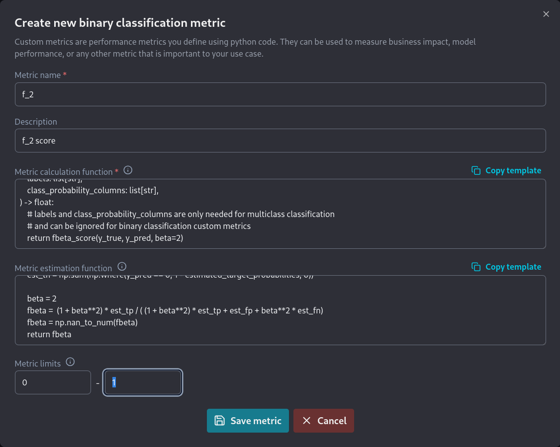
We are then greeted with a new screen where we have to enter the information related to the new metric:
New Custom Binary Classification Metric screen
As shown we need to fill in the following information:
* A name for the metric.
* A short description of the metric.
* A function that calculates the metric.
* A function that estimates the metric
* The numerical limits of the metric, if they exist.
Developing the code for the required functions is described [here](/cloud/model-monitoring/custom-metrics/creating-custom-metrics/writing-functions-for-binary-classification) for the f\_beta score. The required calculation function is:
```python
import numpy as np
import pandas as pd
from sklearn.metrics import fbeta_score
def calculate(
y_true: pd.Series,
y_pred: pd.Series,
y_pred_proba: pd.DataFrame,
chunk_data: pd.DataFrame,
labels: list[str],
class_probability_columns: list[str],
**kwargs
) -> float:
# labels and class_probability_columns are only needed for multiclass classification
# and can be ignored for binary classification custom metrics
return fbeta_score(y_true, y_pred, beta=2)
```
while the required estimation function is:
```python
import numpy as np
import pandas as pd
def estimate(
estimated_target_probabilities: pd.DataFrame,
y_pred: pd.Series,
y_pred_proba: pd.DataFrame,
chunk_data: pd.DataFrame,
labels: list[str],
class_probability_columns: list[str],
**kwargs
) -> float:
# labels and class_probability_columns are only needed for multiclass classification
# and can be ignored for binary classification custom metrics
estimated_target_probabilities = estimated_target_probabilities.to_numpy().ravel()
y_pred = y_pred.to_numpy()
# Create estimated confusion matrix elements
est_tp = np.sum(np.where(y_pred == 1, estimated_target_probabilities, 0))
est_fp = np.sum(np.where(y_pred == 1, 1 - estimated_target_probabilities, 0))
est_fn = np.sum(np.where(y_pred == 0, estimated_target_probabilities, 0))
est_tn = np.sum(np.where(y_pred == 0, 1 - estimated_target_probabilities, 0))
beta = 2
fbeta = (1 + beta**2) * est_tp / ( (1 + beta**2) * est_tp + est_fp + beta**2 * est_fn)
fbeta = np.nan_to_num(fbeta)
return fbeta
```
The default metric limits still apply, so we can leave those as they are. These metric limits ensure that the metric thresholds are constrained to these theoretical limits.\
\
We then fill all this information on the *new binary classification metric* screen:
Completing the new binary classification metric screen
This results in the new metric now being visible in the *Binary Classification* section of the *Custom Metrics* screen.
f_2 binary classification metric
The metric can now be selected for use by any binary classification model from the *Model Settings* page.
{% endtab %}
{% tab title="Multiclass Classification" %}
We click the appropriate *Add new metric* button as seen below:
Adding a new Custom Multiclass Classification Metric
We are then greeted with a new screen where we have to enter the information related to the new metric:
New Custom Multiclass Classification Metric screen
As shown we need to fill in the following information:
* A name for the metric.
* A short description of the metric.
* A function that calculates the metric.
* A function that estimates the metric
* The numerical limits of the metric, if they exist.
Developing the code for the required functions is described [here](/cloud/model-monitoring/custom-metrics/creating-custom-metrics/writing-functions-for-multiclass-classification) for the f\_beta score. The required calculate function is:
```python
import pandas as pd
from sklearn.metrics import fbeta_score
def calculate(
y_true: pd.Series,
y_pred: pd.Series,
y_pred_proba: pd.DataFrame,
chunk_data: pd.DataFrame,
labels: list[str],
class_probability_columns: list[str],
) -> float:
return fbeta_score(y_true, y_pred, beta=2, average='macro')
```
while the required estimate function is:
```python
import numpy as np
import pandas as pd
from sklearn.preprocessing import label_binarize
def estimate(
estimated_target_probabilities: pd.DataFrame,
y_pred: pd.Series,
y_pred_proba: pd.DataFrame,
chunk_data: pd.DataFrame,
labels: list[str],
class_probability_columns: list[str],
):
beta = 2
def estimate_fb(_y_pred, _y_pred_proba, beta) -> float:
# Estimates the Fb metric.
#
# Parameters
# ----------
# y_pred: np.ndarray
# Predicted class label of the sample
# y_pred_proba: np.ndarray
# Probability estimates of the sample for each class in the model.
# beta: float
# beta parameter
#
# Returns
# -------
# metric: float
# Estimated Fb score.
est_tp = np.sum(np.where(_y_pred == 1, _y_pred_proba, 0))
est_fp = np.sum(np.where(_y_pred == 1, 1 - _y_pred_proba, 0))
est_fn = np.sum(np.where(_y_pred == 0, _y_pred_proba, 0))
est_tn = np.sum(np.where(_y_pred == 0, 1 - _y_pred_proba, 0))
fbeta = (1 + beta**2) * est_tp / ( (1 + beta**2) * est_tp + est_fp + beta**2 * est_fn)
fbeta = np.nan_to_num(fbeta)
return fbeta
estimated_target_probabilities = estimated_target_probabilities.to_numpy()
y_preds = label_binarize(y_pred, classes=labels)
ovr_estimates = []
for idx, _ in enumerate(labels):
ovr_estimates.append(
estimate_fb(
y_preds[:, idx],
estimated_target_probabilities[:, idx],
beta=2
)
)
multiclass_metric = np.mean(ovr_estimates)
return multiclass_metric
```
The default metric limits still apply, so we can leave those as they are. These metric limits ensure that the metric thresholds are constrained to these theoretical limits.
We then fill all this information on the new multiclass classification metric screen:
Completing the new multiclass classification metric screen
This results in the new metric now being visible in the *Binary Classification* section of the *Custom Metrics* screen.
F_2 multiclass classification metric
The metric can now be selected for use by any multiclass classification model from the *Model Settings* page.
{% endtab %}
{% tab title="Regression" %}
We click the appropriate *Add new metric* button as seen below:
Adding a new Custom Regression Metric
We are then greeted with a new screen where we have to enter the information related to the new metric:
New Custom Regression Metric screen
As shown we need to fill in the following information:
* A name for the metric.
* A short description of the metric.
* A function that calculates the loss of the metric.
* A function that aggregates the loss results in order to calculate the metric
* The numerical limits of the metric, if they exist.
Developing the code for the required functions is described [here](/cloud/model-monitoring/custom-metrics/creating-custom-metrics/writing-functions-for-regression) for the pinball score. The required loss function is:
```python
import numpy as np
import pandas as pd
def loss(
y_true: pd.Series,
y_pred: pd.Series,
chunk_data: pd.DataFrame,
**kwargs
) -> np.ndarray:
y_true = y_true.to_numpy()
y_pred = y_pred.to_numpy()
alpha = 0.9
factor1 = alpha * np.maximum(y_true - y_pred, 0)
factor2 = (1 - alpha) * np.maximum(y_pred - y_true, 0)
return factor1 + factor2
```
while the required aggregate function is:
```python
import numpy as np
import pandas as pd
def aggregate(
loss: np.ndarray,
chunk_data: pd.DataFrame,
**kwargs
) -> float:
return loss.mean()
```
The default metric limits still apply, so we can leave those as they are. These metric limits ensure that the metric thresholds are constrained to these theoretical limits.
We then fill all this information on the *new regression metric* screen:
Completing the new regression metric screen
This results in the new metric now being visible in the *Regression* section of the *Custom Metrics* screen.
F_2 multiclass classification metric
The metric can now be selected for use by any regression model from the *Model Settings* page.
{% endtab %}
{% endtabs %}
Note that once custom metrics are added they can be selected during the *Add new model* wizard. You can see the relevant step for binary classification in the screenshot below:
Enabling a custom metric during the Add new model wizard.
Custom metrics can also be selected from a model's *settings* page
Selecting Custom Metrics from a model's Performance Settings
# Creating Custom Metrics
How do I create a custom metric
Let's see how we can create a custom metric for each machine learning problem type. To make things more structured, we have created a separate page for each problem type. The key to creating a custom metric is to write the code for its required functions.
## [Creating a Binary Classification Custom Metric](/cloud/model-monitoring/custom-metrics/creating-custom-metrics/writing-functions-for-binary-classification)
## [Creating a Multiclass Classification Custom Metric](/cloud/model-monitoring/custom-metrics/creating-custom-metrics/writing-functions-for-multiclass-classification)
## [Creating a Regression Custom Metric](/cloud/model-monitoring/custom-metrics/creating-custom-metrics/writing-functions-for-regression)
We also discuss more advanced topics such as [handling missing values](/cloud/model-monitoring/custom-metrics/creating-custom-metrics/handling-missing-values) and [creating a custom MTBF metric](/cloud/model-monitoring/custom-metrics/creating-custom-metrics/advanced-tutorial-creating-a-mtbf-custom-metric).
# Writing Functions for Binary Classification
Writing the functions needed to create a custom binary classification metric.
As we have seen on the Introductory [Custom Metric page](/cloud/model-monitoring/custom-metrics) the key components of a custom binary classification metric are the specific Python functions we need to provide for the custom metric to work. Here we will see how to create them.
We will assume the user has access to a Jupyter Notebook running Python with the [NannyML open-source library](https://github.com/NannyML/nannyml) installed.
## Sample Dataset
We have created a sample dataset to facilitate developing the code needed for custom binary classification metrics. The dataset is publicly accessible [here](https://github.com/NannyML/sample_datasets/tree/main/synthetic_pure_covariate_shift_datasets/binary_classification). It is a pure covariate shift dataset that consists of:
* 5 numerical features: `['feature1', 'feature2', 'feature3', 'feature4', 'feature5',]`
* Target column: `y_true`
* Model prediction column: `y_pred`
* The model predicted probability: `y_pred_proba`
* A timestamp column: `timestamp`
* An identifier column: `identifier`
* The probabilities from which the target values have been sampled: `estimated_target_probabilities`
We can inspect the dataset with the following code in a Jupyter cell:
```python
import pandas as pd
import nannyml as nml
reference = pd.read_parquet("https://github.com/NannyML/sample_datasets/raw/main/synthetic_pure_covariate_shift_datasets/binary_classification/synthetic_custom_metrics_binary_classification_reference.pq")
monitored = pd.read_parquet("https://github.com/NannyML/sample_datasets/raw/main/synthetic_pure_covariate_shift_datasets/binary_classification/synthetic_custom_metrics_binary_classification_monitored.pq")
reference.head(5)
```
```markdown
+----+------------+------------+------------+------------+------------+----------+----------------+----------+----------------------------+--------------+----------------------------------+
| | feature1 | feature2 | feature3 | feature4 | feature5 | y_true | y_pred_proba | y_pred | timestamp | identifier | estimated_target_probabilities |
+====+============+============+============+============+============+==========+================+==========+============================+==============+==================================+
| 0 | 0.507982 | 2.10996 | -3.29121 | 2.59278 | 0.970656 | 0 | 0.0208479 | 0 | 2020-03-25 00:00:00 | 60000 | 0.0218986 |
+----+------------+------------+------------+------------+------------+----------+----------------+----------+----------------------------+--------------+----------------------------------+
| 1 | -3.21001 | 2.27251 | -0.0506065 | 0.641354 | 1.82951 | 1 | 0.960223 | 1 | 2020-03-25 00:02:00.960000 | 60001 | 0.959278 |
+----+------------+------------+------------+------------+------------+----------+----------------+----------+----------------------------+--------------+----------------------------------+
| 2 | -0.135355 | 1.13828 | -0.106979 | 0.642139 | -0.647236 | 1 | 0.502806 | 1 | 2020-03-25 00:04:01.920000 | 60002 | 0.507093 |
+----+------------+------------+------------+------------+------------+----------+----------------+----------+----------------------------+--------------+----------------------------------+
| 3 | -2.35321 | -1.0053 | -1.05535 | 1.64436 | 0.251892 | 1 | 0.784257 | 1 | 2020-03-25 00:06:02.880000 | 60003 | 0.785474 |
+----+------------+------------+------------+------------+------------+----------+----------------+----------+----------------------------+--------------+----------------------------------+
| 4 | 0.667785 | 1.38383 | -1.28428 | -0.0995213 | -1.21584 | 0 | 0.121911 | 0 | 2020-03-25 00:08:03.840000 | 60004 | 0.124328 |
+----+------------+------------+------------+------------+------------+----------+----------------+----------+----------------------------+--------------+----------------------------------+
```
## Developing custom binary classification metric functions
NannyML Cloud requires two functions for the custom metric to be used. The first is the `calculate` function, which is mandatory, and is used to calculate realized performance for the custom metric. The second is the `estimate` function, which is optional, and is used to do performance estimation for the custom metric when target values are not available.
### Custom Functions API
The API of these functions is set by NannyML Cloud and is shown as a template on the *New Custom Binary Classification Metric* screen.
```python
import pandas as pd
def calculate(
y_true: pd.Series,
y_pred: pd.Series,
y_pred_proba: pd.DataFrame,
chunk_data: pd.DataFrame,
labels: list[str],
class_probability_columns: list[str],
**kwargs
) -> float:
pass
def estimate(
estimated_target_probabilities: pd.DataFrame,
y_pred: pd.Series,
y_pred_proba: pd.DataFrame,
chunk_data: pd.DataFrame,
labels: list[str],
class_probability_columns: list[str],
**kwargs
) -> float:
pass
```
Creating the `calculate` function is simpler and depends on what we want our custom metric to be. Let's describe the data that are available to us to create our calculate function.
* `y_true`: A `pandas.Series` python object containing the target column.
* `y_pred`: A `pandas.Series` python object containing the model predictions column.
* `y_pred_proba`: A `pandas.DataFrame` python object containing the predicted probabilities column. This is a single-column dataframe for binary classification. It is a dataframe because in multiclass classification it contains multiple columns.
* `chunk_data:` A `pandas.DataFrame` python object containing all columns associated with the model. This allows using other columns in the data provided for the calculation of the custom metric
* `labels`: A python list object containing the values for the class labels. Currently, for binary classification, only 0 and 1 are supported. This parameter is mostly for multiclass classification.
* `class_probability_columns`: A python list object containing the names of the class probability columns. In binary classification, this is a single-element list. This parameter is mostly for multiclass classification.
* `estimated_target_probabilities`: A `pandas.DataFrame` python object containing the calibrated predicted probabilities calculated from the predicted probabilities of the monitored model. This is a single-column dataframe for binary classification. It is a dataframe because in multiclass classification it contains multiple columns.
* `**kwargs`: You can use the keyword arguments placeholder to omit any parameters you don't actually require in your custom metric functions. This keeps your function signatures nice and clean. This also serves as a placeholder for future arguments in later NannyML cloud versions, intended to make the functions forward compatible.
{% hint style="info" %}
Note that `estimated_target_probabilities` are calculated and provided by NannyML. The monitored model's predicted probabilities need not be calibrated for performance estimation to work.\
To simulate this in the dataset we provided this column contains the probabilities from which the target values have been sampled. While using NannyML Cloud however the `estimated_target_probabilities` are estimated from the provided data.
{% endhint %}
### Custom F\_2 score
To create a custom metric from the `F_2` score we would create the `calculate` function below:
```python
import pandas as pd
from sklearn.metrics import fbeta_score
def calculate(
y_true: pd.Series,
y_pred: pd.Series,
y_pred_proba: pd.DataFrame,
chunk_data: pd.DataFrame,
labels: list[str],
class_probability_columns: list[str],
**kwargs
) -> float:
# labels and class_probability_columns are only needed for multiclass classification
# and can be ignored for binary classification custom metrics
return fbeta_score(y_true, y_pred, beta=2)
```
While the `calculate` function of the `F_2` score is straightforward this is not the case for the estimate function. In order to create an estimate function we need to understand performance estimation. Reading [how CBPE works](https://nannyml.readthedocs.io/en/stable/how_it_works/performance_estimation.html#confidence-based-performance-estimation-cbpe) is enough to do so for classification problems. The key concept to understand are the estimated confusion matrix elements and how they are created. We can then use the functional form of the `F_2` score to estimate the metric.
$$
\mathrm{F}\_{\beta} = \frac{(1+\beta^2)\mathrm{TP}}{(1+\beta^2)\mathrm{TP}+\mathrm{FP}+\beta^2\mathrm{FN}}
$$
Putting everything together we get:
```python
import numpy as np
import pandas as pd
def estimate(
estimated_target_probabilities: pd.DataFrame,
y_pred: pd.Series,
y_pred_proba: pd.DataFrame,
chunk_data: pd.DataFrame,
labels: list[str],
class_probability_columns: list[str],
**kwargs
) -> float:
# labels and class_probability_columns are only needed for multiclass classification
# and can be ignored for binary classification custom metrics
estimated_target_probabilities = estimated_target_probabilities.to_numpy().ravel()
y_pred = y_pred.to_numpy()
# Create estimated confusion matrix elements
est_tp = np.sum(np.where(y_pred == 1, estimated_target_probabilities, 0))
est_fp = np.sum(np.where(y_pred == 1, 1 - estimated_target_probabilities, 0))
est_fn = np.sum(np.where(y_pred == 0, estimated_target_probabilities, 0))
est_tn = np.sum(np.where(y_pred == 0, 1 - estimated_target_probabilities, 0))
beta = 2
fbeta = (1 + beta**2) * est_tp / ( (1 + beta**2) * est_tp + est_fp + beta**2 * est_fn)
fbeta = np.nan_to_num(fbeta)
return fbeta
```
We can test those functions on the dataset loaded earlier. Assuming we run the functions as provided in a Jupyter cell we can then call them. Running `calculate` we get:
```python
class_probability_columns = ['y_pred_proba',]
labels = [0, 1]
estimate(
reference[['estimated_target_probabilities']],
reference['y_pred'],
reference[class_probability_columns],
reference,
labels=labels,
class_probability_columns=class_probability_columns
)
```
```python
0.8082738516020327
```
While running `estimate` we get:
```python
calculate(
reference['y_true'],
reference['y_pred'],
reference[class_probability_columns],
reference,
labels=labels,
class_probability_columns=class_probability_columns
)
```
```python
0.8087246321117878
```
We can see that the values between estimated and realized `F_2` score are very close. This means that we are likely estimating the metric correctly. The values will never match due to the statistical nature of the problem. Sampling error will always induce some differences.
## Testing a Custom Metric in the Cloud product
We saw how to add a binary classification custom metric in the [*Custom Metrics Introductory* page](/cloud/model-monitoring/custom-metrics). We can further test it by using the dataset in the cloud product. The datasets are publicly available hence we can use the Public Link option when adding data to a new model.
Reference Dataset Public Link:
```url
https://github.com/NannyML/sample_datasets/raw/main/synthetic_pure_covariate_shift_datasets/binary_classification/synthetic_custom_metrics_binary_classification_reference.pq
```
Monitored Dataset Public Link:
```url
https://github.com/NannyML/sample_datasets/raw/main/synthetic_pure_covariate_shift_datasets/binary_classification/synthetic_custom_metrics_binary_classification_monitored.pq
```
The process of creating a new model is described in the [Monitoring a tabular data model](/cloud/model-monitoring/tutorials/monitoring-a-tabular-data-model).
We need to be careful to mark `estimated_target_probabilities` as an **ignored column** since it's related to our oracle knowledge of the problem and not to the monitored model the dataset represents.
Ignoring the data column containing estimated_target_probabilities
Note that when we are on the *Metrics* page
Metrics page of the Add new model Wizard
we can go to *Performance monitoring* and directly add a custom metric we have already specified.
Performance settings of the Metrics page of the Add new model Wizard
After the model has been added to NannyML Cloud and the first run has been completed we can inspect the monitoring results. Of particular interest to us is the comparison between estimated and realized performance for our custom metric.
We see that NannyML can accurately estimate our custom metric across the whole dataset. Even in the areas where there is a performance difference. This means that our calculate and estimate functions have been correctly created as the dataset is created specifically to facilitate this test.
You may have noticed that for custom metrics we don't have a sampling error implementation. Therefore you will have to make a qualitative judgement, based on the results, whether the estimated and realized performance results are a good enough match or not.
## Next Steps
You are now ready to use your new custom metric in production. However, you may want to make your implementation more robust to account for the data you will encounter in production. For example, you can [add missing value handling](/cloud/model-monitoring/custom-metrics/creating-custom-metrics/handling-missing-values) to your implementation.
# Writing Functions for Multiclass Classification
Writing the functions needed to create a custom multiclass classification metric.
As we have seen on the Introductory [Custom Metric page](/cloud/model-monitoring/custom-metrics) the key components of a custom multiclass classification metric are the specific Python functions we need to provide for the custom metric to work. Here we will see how to create them.
We will assume the user has access to a Jupyter Notebook running Python with the [NannyML open-source library](https://github.com/NannyML/nannyml) installed.
## Sample Dataset
We have created a sample dataset to facilitate developing the code needed for custom binary classification metrics. The dataset is publicly accessible [here](https://github.com/NannyML/sample_datasets/tree/main/synthetic_pure_covariate_shift_datasets/multiclass_classification). It is a pure covariate shift dataset that consists of:
* 7 numerical features: `['feature1', 'feature2', 'feature3', 'feature4', 'feature5', 'feature6', 'feature7']`
* Target column that contains the 5 classes `{0,1,2,3,4}`: `y_true`
* Model prediction column: `y_pred`
* The model predicted probability columns: `y_pred_proba_0/1/2/3/4`
* A timestamp column: `timestamp`
* An identifier column: `identifier`
* The probabilities from which the target values have been sampled: `estimated_target_probabilities_0/1/2/3/4`
We can inspect the dataset with the following code in a Jupyter cell:
```python
import pandas as pd
import nannyml as nml
reference = pd.read_parquet("https://github.com/NannyML/sample_datasets/raw/main/synthetic_pure_covariate_shift_datasets/multiclass_classification/synthetic_custom_metrics_multiclass_classification_reference.pq")
monitored = pd.read_parquet("https://github.com/NannyML/sample_datasets/raw/main/synthetic_pure_covariate_shift_datasets/multiclass_classification/synthetic_custom_metrics_multiclass_classification_monitored.pq")
reference.head(5)
```
## Developing custom multiclass classification metric functions
NannyML Cloud requires two functions for the custom metric to be used. The first is the `calculate` function, which is mandatory, and is used to calculate realized performance for the custom metric. The second is the `estimate` function, which is optional, and is used to do performance estimation for the custom metric when target values are not available.
### Custom Functions API
The API of these functions is set by NannyML Cloud and is shown as a template on the *New Custom Multiclass Classification Metric* screen. They are the same for both binary and multiclass classification.
```python
import pandas as pd
def calculate(
y_true: pd.Series,
y_pred: pd.Series,
y_pred_proba: pd.DataFrame,
chunk_data: pd.DataFrame,
labels: list[str],
class_probability_columns: list[str],
**kwargs
) -> float:
pass
def estimate(
estimated_target_probabilities: pd.DataFrame,
y_pred: pd.Series,
y_pred_proba: pd.DataFrame,
chunk_data: pd.DataFrame,
labels: list[str],
class_probability_columns: list[str],
**kwargs,
) -> float:
pass
```
Creating the `calculate` function is simpler and depends on what we want our custom metric to be. Let's describe the data that are available to us to create our calculate function.
* `y_true`: A `pandas.Series` python object containing the target column.
* `y_pred`: A `pandas.Series` python object containing the model predictions column.
* `y_pred_proba`: A `pandas.DataFrame` python object containing the predicted probabilities column. This is a single-column dataframe for binary classification. It is a dataframe because in multiclass classification it contains multiple columns.
* `chunk_data:` A `pandas.DataFrame` python object containing all columns associated with the model. This allows using other columns in the data provided for the calculation of the custom metric
* `labels`: A python list object containing the values for the class labels. Currently, for binary classification, only 0 and 1 are supported. This parameter is mostly for multiclass classification.
* `class_probability_columns`: A python list object containing the names of the class probability columns. The column names of the `class_probability_columns` and `y_pred_proba` dataframes are the elements of this list. This helps ensure that the column referring to the appropriate class label is always selected.
* `estimated_target_probabilities`: A `pandas.DataFrame` python object containing the calibrated predicted probabilities calculated from the predicted probabilities of the monitored model. This is a single-column dataframe for binary classification. It is a dataframe because in multiclass classification it contains multiple columns.
* `**kwargs`: You can use the keyword arguments placeholder to omit any parameters you don't actually require in your custom metric functions. This keeps your function signatures nice and clean. This also serves as a placeholder for future arguments in later NannyML cloud versions, intended to make the functions forward compatible.
{% hint style="info" %}
Note that `estimated_target_probabilities` are calculated and provided by NannyML. The monitored model's predicted probabilities need not be calibrated for performance estimation to work.\
To simulate this in the dataset we provided this column contains the probabilities from which the target values have been sampled. While using NannyML Cloud however the `estimated_target_probabilities` are estimated from the provided data.
{% endhint %}
### Custom F\_2 score
To create a custom metric from the `F_2` score we would create the `calculate` function below:
```python
import pandas as pd
from sklearn.metrics import fbeta_score
def calculate(
y_true: pd.Series,
y_pred: pd.Series,
y_pred_proba: pd.DataFrame,
chunk_data: pd.DataFrame,
labels: list[str],
class_probability_columns: list[str],
**kwargs
) -> float:
return fbeta_score(y_true, y_pred, beta=2, average='macro')
```
While the `calculate` function of the `F_2` score is straightforward this is not the case for the estimate function. In order to create an estimate function we need to understand performance estimation. Reading [how CBPE works](https://nannyml.readthedocs.io/en/stable/how_it_works/performance_estimation.html#confidence-based-performance-estimation-cbpe) is enough to do so for classification problems. The key concept to understand are the estimated confusion matrix elements and how they are created. We can then use the functional form of the `F_2` score to estimate the metric.
$$
\mathrm{F}\_{\beta} = \frac{(1+\beta^2)\mathrm{TP}}{(1+\beta^2)\mathrm{TP}+\mathrm{FP}+\beta^2\mathrm{FN}}
$$
Lastly, we need to consider how to average the class results. We will use macro averaging. Putting everything together we get:
```python
import numpy as np
import pandas as pd
from sklearn.preprocessing import label_binarize
def estimate(
estimated_target_probabilities: pd.DataFrame,
y_pred: pd.Series,
y_pred_proba: pd.DataFrame,
chunk_data: pd.DataFrame,
labels: list[str],
class_probability_columns: list[str],
**kwargs
):
beta = 2
def estimate_fb(_y_pred, _y_pred_proba, beta) -> float:
# Estimates the Fb metric.
#
# Parameters
# ----------
# y_pred: np.ndarray
# Predicted class label of the sample
# y_pred_proba: np.ndarray
# Probability estimates of the sample for each class in the model.
# beta: float
# beta parameter
#
# Returns
# -------
# metric: float
# Estimated Fb score.
est_tp = np.sum(np.where(_y_pred == 1, _y_pred_proba, 0))
est_fp = np.sum(np.where(_y_pred == 1, 1 - _y_pred_proba, 0))
est_fn = np.sum(np.where(_y_pred == 0, _y_pred_proba, 0))
est_tn = np.sum(np.where(_y_pred == 0, 1 - _y_pred_proba, 0))
fbeta = (1 + beta**2) * est_tp / ( (1 + beta**2) * est_tp + est_fp + beta**2 * est_fn)
fbeta = np.nan_to_num(fbeta)
return fbeta
estimated_target_probabilities = estimated_target_probabilities.to_numpy()
y_preds = label_binarize(y_pred, classes=labels)
ovr_estimates = []
for idx, _ in enumerate(labels):
ovr_estimates.append(
estimate_fb(
y_preds[:, idx],
estimated_target_probabilities[:, idx],
beta=2
)
)
multiclass_metric = np.mean(ovr_estimates)
return multiclass_metric
```
We can test those functions on the dataset loaded earlier. Assuming we run the functions as provided in a Jupyter cell we can then call them. Running `calculate` we get:
```python
features = ['feature1', 'feature2', 'feature3', 'feature4', 'feature5', 'feature6', 'feature7']
class_probability_columns = ['y_pred_proba_0', 'y_pred_proba_1', 'y_pred_proba_2', 'y_pred_proba_3', 'y_pred_proba_4',]
labels = [0, 1, 2, 3, 4]
estimated_target_probabilties = [
'estimated_target_probabilities_0',
'estimated_target_probabilities_1',
'estimated_target_probabilities_2',
'estimated_target_probabilities_3',
'estimated_target_probabilities_4'
]
# simulate estimated_target_probabilities and y_pred_proba having the same column names
estimated_target_probabilities = reference[estimated_target_probabilties].rename(
columns=dict(zip(estimated_target_probabilties, class_probability_columns))
)
estimate(
estimated_target_probabilities=estimated_target_probabilities,
y_pred=reference['y_pred'],
y_pred_proba=reference[class_probability_columns],
chunk_data=reference,
labels=labels,
class_probability_columns=class_probability_columns
)
```
```python
0.6929117226840699
```
While running `estimate` we get:
```python
calculate(
y_true=reference['y_true'],
y_pred=reference['y_pred'],
y_pred_proba=reference[class_probability_columns],
chunk_data=reference,
labels=labels,
class_probability_columns=class_probability_columns
)
```
```python
0.694377528321876
```
We can see that the values between estimated and realized `F_2` score are very close. This means that we are likely estimating the metric correctly. The values will never match due to the statistical nature of the problem. Sampling error will always induce some differences.
## Testing a Custom Metric in the Cloud product
We saw how to add a multiclass classification custom metric in the [Custom Metrics Introductory page](/cloud/model-monitoring/custom-metrics). We can further test it by using the dataset in the cloud product. The datasets are publicly available hence we can use the Public Link option when adding data to a new model.
Reference Dataset Public Link:
```url
https://github.com/NannyML/sample_datasets/raw/main/synthetic_pure_covariate_shift_datasets/multiclass_classification/synthetic_custom_metrics_multiclass_classification_reference.pq
```
Monitored Dataset Public Link:
```url
https://github.com/NannyML/sample_datasets/raw/main/synthetic_pure_covariate_shift_datasets/multiclass_classification/synthetic_custom_metrics_multiclass_classification_monitored.pq
```
The process of creating a new model is described in the [Monitoring a tabular data model](/cloud/model-monitoring/tutorials/monitoring-a-tabular-data-model).
We need to be careful to mark `estimated_target_probabilities` columns as an **ignored column** since it's related to our oracle knowledge of the problem and not to the monitored model the dataset represents.
Ignoring the data column containing estimated_target_probabilities
Note that when we are on the *Metrics* page
Metrics page of the Add new model Wizard
we can go to *Performance monitoring* and directly add a custom metric we have already specified.
Performance settings of the Metrics page of the Add new model Wizard
After the model has been added to NannyML Cloud and the first run has been completed we can inspect the monitoring results. Of particular interest to us is the comparison between estimated and realized performance for our custom metric.
We see that NannyML can accurately estimate our custom metric across the whole dataset. Even in the areas where there is a performance difference. This means that our calculate and estimate functions have been correctly created as the dataset is created specifically to facilitate this test.
You may have noticed that for custom metrics we don't have a sampling error implementation. Therefore you will have to make a qualitative judgement, based on the results, whether the estimated and realized performance results are a good enough match or not.
## Next Steps
You are now ready to use your new custom metric in production. However, you may want to make your implementation more robust to account for the data you will encounter in production. For example, you can [add missing value handling](/cloud/model-monitoring/custom-metrics/creating-custom-metrics/handling-missing-values) to your implementation.
# Writing Functions for Regression
Writing the functions needed to create a custom regression metric.
As we have seen on the Introductory [Custom Metric page](/cloud/model-monitoring/custom-metrics) the key components of a custom binary classification metric are the specific Python functions we need to provide for the custom metric to work. Here we will see how to create them.
We will assume the user has access to a Jupyter Notebook running Python with the [NannyML open-source library](https://github.com/NannyML/nannyml) installed.
## Sample Dataset
We have created a sample dataset to facilitate developing the code needed for custom binary classification metrics. The dataset is publicly accessible [here](https://github.com/NannyML/sample_datasets/tree/main/synthetic_pure_covariate_shift_datasets/regression). It is a pure covariate shift dataset that consists of:
* 7 numerical features: `['feature1', 'feature2', 'feature3', 'feature4', 'feature5', 'feature6', 'feature7']`
* Target column: `y_true`
* Model prediction column: `y_pred`
* A timestamp column: `timestamp`
* An identifier column: `identifier`
We can inspect the dataset with the following code in a Jupyter cell:
```python
import pandas as pd
import nannyml as nml
reference = pd.read_parquet("https://github.com/NannyML/sample_datasets/raw/main/synthetic_pure_covariate_shift_datasets/regression/synthetic_custom_metrics_regression_reference.pq")
monitored = pd.read_parquet("https://github.com/NannyML/sample_datasets/raw/main/synthetic_pure_covariate_shift_datasets/regression/synthetic_custom_metrics_regression_monitored.pq")
reference.head(5)
```
```markdown
+----+------------+------------+------------+------------+------------+------------+------------+----------+----------+----------------------------+
| | feature1 | feature2 | feature3 | feature4 | feature5 | feature6 | feature7 | y_true | y_pred | timestamp |
+====+============+============+============+============+============+============+============+==========+==========+============================+
| 0 | 0.899145 | -2.64707 | 2.80074 | 2.02636 | -2.53157 | -2.12171 | -0.360711 | 7.97047 | 3.15523 | 2020-03-11 00:00:00 |
+----+------------+------------+------------+------------+------------+------------+------------+----------+----------+----------------------------+
| 1 | -1.09015 | -0.442365 | 1.94911 | -0.378131 | 0.517571 | 2.67345 | -1.71358 | -13.5075 | -13.1339 | 2020-03-11 00:01:40.800000 |
+----+------------+------------+------------+------------+------------+------------+------------+----------+----------+----------------------------+
| 2 | 0.619741 | 0.924163 | 1.30714 | 2.60199 | -0.776712 | 1.41447 | -0.848892 | -6.39705 | -5.324 | 2020-03-11 00:03:21.600000 |
+----+------------+------------+------------+------------+------------+------------+------------+----------+----------+----------------------------+
| 3 | -1.7384 | -0.54207 | 1.58942 | 4.12909 | -1.78157 | -0.275194 | -1.82792 | -11.8357 | -3.20461 | 2020-03-11 00:05:02.400000 |
+----+------------+------------+------------+------------+------------+------------+------------+----------+----------+----------------------------+
| 4 | -4.78688 | 0.330358 | -2.56052 | -2.32385 | 1.19089 | -2.58183 | -1.68192 | 4.17999 | 5.68762 | 2020-03-11 00:06:43.200000 |
+----+------------+------------+------------+------------+------------+------------+------------+----------+----------+----------------------------+
```
## Developing custom regression metric functions
NannyML Cloud requires two functions for the custom metric to be used. The first is the `loss` function used to calculate the instance level loss. The second is the `aggregate` function used to aggregate over the instance level results. We are using this decomposition to be able to use the [Direct Loss Estimation](https://nannyml.readthedocs.io/en/stable/how_it_works/performance_estimation.html#direct-loss-estimation-dle) algorithm for performance estimation. In realized performance loss is calculated while in estimated performance loss is estimated.
### Custom Functions API
The API of these functions is set by NannyML Cloud and is shown as a template on the *New Custom Regression Metric* screen.
```python
import numpy as np
import pandas as pd
def loss(
y_true: pd.Series,
y_pred: pd.Series,
chunk_data: pd.DataFrame,
**kwargs
) -> np.ndarray:
pass
def aggregate(
loss: np.ndarray,
chunk_data: pd.DataFrame,
**kwargs
) -> float:
pass
```
Let's use the [pinball metric](https://scikit-learn.org/stable/modules/model_evaluation.html#pinball-loss) as our custom regression metric. We start with creating the `loss` function. Let's describe the data that are available to us to create our calculate function.
* `y_true`: A `pandas.Series` python object containing the target column.
* `y_pred`: A `pandas.Series` python object containing the model predictions column.
* `chunk_data:` A `pandas.DataFrame` python object containing all columns associated with the model. This allows using other columns in the data provided for the calculation of the custom metric
### Custom Pinball metric
We will create a custom metric from the pinball loss. Let's use an `alpha` value of `0.9`. The `loss` function would be:
```python
import numpy as np
import pandas as pd
def loss(
y_true: pd.Series,
y_pred: pd.Series,
chunk_data: pd.DataFrame,
**kwargs
) -> np.ndarray:
y_true = y_true.to_numpy()
y_pred = y_pred.to_numpy()
alpha = 0.9
factor1 = alpha * np.maximum(y_true - y_pred, 0)
factor2 = (1 - alpha) * np.maximum(y_pred - y_true, 0)
return factor1 + factor2
```
The `aggregate` function is quite simpler:
```python
import numpy as np
import pandas as pd
def aggregate(
loss: np.ndarray,
chunk_data: pd.DataFrame,
**kwargs
) -> float:
return loss.mean()
```
We can test those functions on the dataset loaded earlier. Assuming we run the functions as provided in a Jupyter cell we can then call them. Running them we get:
```python
loss = loss(
y_true=reference['y_true'],
y_pred=reference['y_pred'],
chunk_data=reference,
)
aggregate(
loss=_loss,
chunk_data=reference,
)
```
```python
0.6298987071792433
```
We can double check the result with `sklearn`:
```python
from sklearn.metrics import mean_pinball_loss
mean_pinball_loss(y_true=reference.y_true, y_pred=reference.y_pred, alpha=0.9)
```
```python
0.6298987071792433
```
The results match as expected meaning we have correctly specified our custom metric.
## Testing a Custom Metric in the Cloud product
We saw how to add a binary classification custom metric in the [Custom Metrics Introductory page](/cloud/model-monitoring/custom-metrics). We can further test it by using the dataset in the cloud product. The datasets are publicly available hence we can use the Public Link option when adding data to a new model.
Reference Dataset Public Link:
```url
https://github.com/NannyML/sample_datasets/raw/main/synthetic_pure_covariate_shift_datasets/regression/synthetic_custom_metrics_regression_reference.pq
```
Monitored Dataset Public Link:
```url
https://github.com/NannyML/sample_datasets/raw/main/synthetic_pure_covariate_shift_datasets/regression/synthetic_custom_metrics_regression_monitored.pq
```
The process of creating a new model is described in the [Monitoring a tabular data model](/cloud/model-monitoring/tutorials/monitoring-a-tabular-data-model).
Note that when we are on the **Metrics** page
Metrics page of the Add new model Wizard
we can go to *Performance monitoring* and directly add a custom metric we have already specified.
Performance settings of the Metrics page of the Add new model Wizard
After the model has been added to NannyML Cloud and the first run has been completed we can inspect the monitoring results. Of particular interest to us is the comparison between estimated and realized performance for our custom metric.
We see that NannyML can accurately estimate our custom metric across the whole dataset. Even in the areas where there is a performance difference. This means that our `loss` function is compatible with DLE and we can reliably use both performance calculation and performance estimation for our custom metric.
You may have noticed that for custom metrics we don't have a sampling error implementation. Therefore you will have to make a qualitative judgement, based on the results, whether the estimated and realized performance results are a good enough match or not.
## Next Steps
You are now ready to use your new custom metric in production. However, you may want to make your implementation more robust to account for the data you will encounter in production. For example, you can [add missing value handling](/cloud/model-monitoring/custom-metrics/creating-custom-metrics/handling-missing-values) to your implementation.
# Handling Missing Values
Advanced Tutorial. Handling missing values with your custom metric functions.
In previous tutorials, we saw how to create the functions needed for simple custom metrics for [binary classification](/cloud/model-monitoring/custom-metrics/creating-custom-metrics/writing-functions-for-binary-classification), [multiclass classification](/cloud/model-monitoring/custom-metrics/creating-custom-metrics/writing-functions-for-multiclass-classification), and [regression](/cloud/model-monitoring/custom-metrics/creating-custom-metrics/writing-functions-for-regression). Let's see how we can improve on said code to be able to handle missing values in our data. As previously we assume the user has access to a Jupyter Notebook python environment with the [NannyML open-source](https://github.com/NannyML/nannyml) library installed.
## Handling missing values in binary classification
Let's load the covariate shift dataset we have been using and add some missing values.
```python
import numpy as np
import pandas as pd
import nannyml as nml
# Comment out if needed the code below to filter out warnings
# import warnings
# warnings.filterwarnings('ignore')
# Comment out if needed the code below to see logging messages
# import logging
# logging.basicConfig(level=logging.DEBUG)
reference = pd.read_parquet("https://github.com/NannyML/sample_datasets/raw/main/synthetic_pure_covariate_shift_datasets/binary_classification/synthetic_custom_metrics_binary_classification_reference.pq")
monitored = pd.read_parquet("https://github.com/NannyML/sample_datasets/raw/main/synthetic_pure_covariate_shift_datasets/binary_classification/synthetic_custom_metrics_binary_classification_monitored.pq")
reference.y_pred.iloc[11_000:13_000] = np.nan
reference.y_true.iloc[17_000:19_000] = np.nan
reference.y_pred.iloc[21_000:23_000] = np.nan
reference.y_true.iloc[27_000:29_000] = np.nan
reference.y_pred.iloc[31_000:33_000] = np.nan
reference.y_true.iloc[37_000:39_000] = np.nan
reference.y_pred_proba.iloc[17_000:19_000] = np.nan
reference.y_pred_proba.iloc[27_000:29_000] = np.nan
reference.y_pred_proba.iloc[37_000:39_000] = np.nan
```
As a reminder here are the custom metric functions for the `F_2` metric we [already created](/cloud/model-monitoring/custom-metrics/creating-custom-metrics/writing-functions-for-binary-classification).
```python
import pandas as pd
from sklearn.metrics import fbeta_score
def calculate(
y_true: pd.Series,
y_pred: pd.Series,
y_pred_proba: pd.DataFrame,
chunk_data: pd.DataFrame,
labels: list[str],
class_probability_columns: list[str],
**kwargs
) -> float:
# labels and class_probability_columns are only needed for multiclass classification
# and can be ignored for binary classification custom metrics
return fbeta_score(y_true, y_pred, beta=2)
```
```python
import numpy as np
import pandas as pd
def estimate(
estimated_target_probabilities: pd.DataFrame,
y_pred: pd.Series,
y_pred_proba: pd.DataFrame,
chunk_data: pd.DataFrame,
labels: list[str],
class_probability_columns: list[str],
**kwargs
) -> float:
# labels and class_probability_columns are only needed for multiclass classification
# and can be ignored for binary classification custom metrics
estimated_target_probabilities = estimated_target_probabilities.to_numpy().ravel()
y_pred = y_pred.to_numpy()
# Create estimated confusion matrix elements
est_tp = np.sum(np.where(y_pred == 1, estimated_target_probabilities, 0))
est_fp = np.sum(np.where(y_pred == 1, 1 - estimated_target_probabilities, 0))
est_fn = np.sum(np.where(y_pred == 0, estimated_target_probabilities, 0))
est_tn = np.sum(np.where(y_pred == 0, 1 - estimated_target_probabilities, 0))
beta = 2
fbeta = (1 + beta**2) * est_tp / ( (1 + beta**2) * est_tp + est_fp + beta**2 * est_fn)
fbeta = np.nan_to_num(fbeta)
return fbeta
```
There is an open question of how to deal with the missing values. This is ultimately up to the user and the particular use case for which the custom metric is being created. Here we will show how to remove rows containing missing values for the custom metric calculation. Doing this the custom metric functions become:
```python
import pandas as pd
from sklearn.metrics import fbeta_score
def calculate(
y_true: pd.Series,
y_pred: pd.Series,
y_pred_proba: pd.DataFrame,
chunk_data: pd.DataFrame,
**kwargs
) -> float:
data = pd.DataFrame({
'y_true': y_true,
'y_pred': y_pred
})
data.dropna(axis=0, inplace=True)
return fbeta_score(data.y_true, data.y_pred, beta=2)
```
```python
import numpy as np
import pandas as pd
def estimate(
estimated_target_probabilities: pd.DataFrame,
y_pred: pd.Series,
y_pred_proba: pd.DataFrame,
chunk_data: pd.DataFrame,
labels: list[str],
class_probability_columns: list[str],
) -> float:
# labels and class_probability_columns are only needed for multiclass classification
# and can be ignored for binary classification custom metrics
data = pd.DataFrame({
'estimated_target_probabilities': estimated_target_probabilities.to_numpy().ravel(),
'y_pred_proba': y_pred_proba.to_numpy().ravel(),
'y_pred': y_pred,
})
data.dropna(axis=0, inplace=True)
y_pred = data.y_pred.to_numpy()
estimated_target_probabilities = data.estimated_target_probabilities.to_numpy()
est_tp = np.sum(np.where(y_pred == 1, estimated_target_probabilities, 0))
est_fp = np.sum(np.where(y_pred == 1, 1 - estimated_target_probabilities, 0))
est_fn = np.sum(np.where(y_pred == 0, estimated_target_probabilities, 0))
est_tn = np.sum(np.where(y_pred == 0, 1 - estimated_target_probabilities, 0))
beta = 2
fbeta = (1 + beta**2) * est_tp / ( (1 + beta**2) * est_tp + est_fp + beta**2 * est_fn)
fbeta = np.nan_to_num(fbeta)
return fbeta
```
By looking at the `estimate` function it is visible that even there, decisions may need to be made. For example which columns to include in the functions that drops rows if they contain missing values. Again this can depend on the use case and what data the function is expected to handle.
We can now test our functions to see if they are robust when they encounter missing values:
```python
class_probability_columns = ['y_pred_proba',]
labels = [0, 1]
calculate(
reference['y_true'],
reference['y_pred'],
reference[class_probability_columns],
reference,
labels=labels,
class_probability_columns=class_probability_columns
)
```
```python
0.8081988545474137
```
```python
estimate(
reference[['estimated_target_probabilities']],
reference['y_pred'],
reference[class_probability_columns],
reference,
labels=labels,
class_probability_columns=class_probability_columns
)
```
```python
0.8081160256970812
```
## Next Steps
We can now test our new functions by creating a new custom metric either through the [GUI of the web interface](/cloud/model-monitoring/custom-metrics) or by using the [NannyML Cloud SDK](/cloud/model-monitoring/custom-metrics/adding-a-custom-metric-through-nannyml-sdk).
# Advanced Tutorial: Creating a MTBF Custom Metric
Creating a MTBF custom metric using the timestamp column from chunk data.
Often we will need to create more complicated custom metrics. Let's use [Mean Time Between Failures](https://en.wikipedia.org/wiki/Mean_time_between_failures) as an example. In order to calculate it we will need information from columns in the chunk data dataframe.
We will assume the user has access to a Jupyter Notebook running Python with the [NannyML open-source library](https://github.com/NannyML/nannyml) installed.
## Repurposing our binary classification sample dataset
We will be using the same dataset we saw when [writing custom metric functions for binary classification](/cloud/model-monitoring/custom-metrics/creating-custom-metrics/writing-functions-for-binary-classification). The dataset is publicly accessible [here](https://github.com/NannyML/sample_datasets/tree/main/synthetic_pure_covariate_shift_datasets/binary_classification). It is a pure covariate shift dataset that consists of:
* 5 numerical features: `['feature1', 'feature2', 'feature3', 'feature4', 'feature5',]`
* Target column: `y_true`
* Model prediction column: `y_pred`
* The model predicted probability: `y_pred_proba`
* A timestamp column: `timestamp`
* An identifier column: `identifier`
* The probabilities from which the target values have been sampled: `estimated_target_probabilities`
Here the meaning of the dataset will be a little different. We have some machines operating over a time period. We are also performing regular checks on them to see if there are any failures. We can aggregate our results over this time period to see how many failures we observed over that period compared to the total operating time of all machines inspected during this period. This will be our simple MTBF metric.
We can inspect the dataset with the following code in a Jupyter cell:
```python
import pandas as pd
import nannyml as nml
reference = pd.read_parquet("https://github.com/NannyML/sample_datasets/raw/main/synthetic_pure_covariate_shift_datasets/binary_classification/synthetic_custom_metrics_binary_classification_reference.pq")
monitored = pd.read_parquet("https://github.com/NannyML/sample_datasets/raw/main/synthetic_pure_covariate_shift_datasets/binary_classification/synthetic_custom_metrics_binary_classification_monitored.pq")
reference.head(5)
```
```markdown
+----+------------+------------+------------+------------+------------+----------+----------------+----------+----------------------------+--------------+----------------------------------+
| | feature1 | feature2 | feature3 | feature4 | feature5 | y_true | y_pred_proba | y_pred | timestamp | identifier | estimated_target_probabilities |
+====+============+============+============+============+============+==========+================+==========+============================+==============+==================================+
| 0 | 0.507982 | 2.10996 | -3.29121 | 2.59278 | 0.970656 | 0 | 0.0208479 | 0 | 2020-03-25 00:00:00 | 60000 | 0.0218986 |
+----+------------+------------+------------+------------+------------+----------+----------------+----------+----------------------------+--------------+----------------------------------+
| 1 | -3.21001 | 2.27251 | -0.0506065 | 0.641354 | 1.82951 | 1 | 0.960223 | 1 | 2020-03-25 00:02:00.960000 | 60001 | 0.959278 |
+----+------------+------------+------------+------------+------------+----------+----------------+----------+----------------------------+--------------+----------------------------------+
| 2 | -0.135355 | 1.13828 | -0.106979 | 0.642139 | -0.647236 | 1 | 0.502806 | 1 | 2020-03-25 00:04:01.920000 | 60002 | 0.507093 |
+----+------------+------------+------------+------------+------------+----------+----------------+----------+----------------------------+--------------+----------------------------------+
| 3 | -2.35321 | -1.0053 | -1.05535 | 1.64436 | 0.251892 | 1 | 0.784257 | 1 | 2020-03-25 00:06:02.880000 | 60003 | 0.785474 |
+----+------------+------------+------------+------------+------------+----------+----------------+----------+----------------------------+--------------+----------------------------------+
| 4 | 0.667785 | 1.38383 | -1.28428 | -0.0995213 | -1.21584 | 0 | 0.121911 | 0 | 2020-03-25 00:08:03.840000 | 60004 | 0.124328 |
+----+------------+------------+------------+------------+------------+----------+----------------+----------+----------------------------+--------------+----------------------------------+
```
## Developing the MTBF metric functions
NannyML Cloud requires two functions for the custom metric to be used. The first is the `calculate` function, which is mandatory, and is used to calculate realized performance for the custom metric. The second is the `estimate` function, which is optional, and is used to do performance estimation for the custom metric when target values are not available.
To create a custom metric from the `MTBF` metric we create the `calculate` function below:
```python
import pandas as pd
def calculate(
y_true: pd.Series,
y_pred: pd.Series,
y_pred_proba: pd.DataFrame,
chunk_data: pd.DataFrame,
**kwargs
) -> float:
_max = chunk_data['timestamp'].max()
_min = chunk_data['timestamp'].min()
hours = len(y_true) * (_max - _min).seconds / 3600
failures = y_true.sum()
return hours/failures
```
The `estimate` function is relatively straightforward in our case. We can estimate the number of failures by using the sum of `estimated_target_probabilities`. Hence we get:
```python
import pandas as pd
def estimate(
estimated_target_probabilities: pd.DataFrame,
y_pred: pd.Series,
y_pred_proba: pd.DataFrame,
chunk_data: pd.DataFrame,
**kwargs
) -> float:
_max = chunk_data['timestamp'].max()
_min = chunk_data['timestamp'].min()
hours = len(y_pred) * (_max - _min).seconds / 3600
failures = estimated_target_probabilities.sum()
return (hours/failures)[0]
```
We can test those functions on the dataset loaded earlier. Assuming we run the functions as provided in a Jupyter cell we can then call them. Running `calculate` we get:
```python
class_probability_columns = ['y_pred_proba',]
labels = [0, 1]
estimate(
reference[['estimated_target_probabilities']],
reference['y_pred'],
reference[class_probability_columns],
reference,
labels=labels,
class_probability_columns=class_probability_columns
)
```
```python
47.75475389197522
```
While running `estimate` we get:
```python
calculate(
reference['y_true'],
reference['y_pred'],
reference[class_probability_columns],
reference,
labels=labels,
class_probability_columns=class_probability_columns
)
```
```python
47.57281018074348
```
We can see that the values between estimated and realized `MTBF` score are very close. This means that we are likely estimating the metric correctly. The values will never match due to the statistical nature of the problem. Sampling error will always induce some differences.
## Testing MTBF in the Cloud product
We saw how to add a binary classification custom metric in the [Custom Metrics Introductory page](/cloud/model-monitoring/custom-metrics). We can further test it by using the dataset in the cloud product. The datasets are publically available hence we can use the Public Link option when adding data to a new model.
Reference Dataset Public Link:
```url
https://github.com/NannyML/sample_datasets/raw/main/synthetic_pure_covariate_shift_datasets/binary_classification/synthetic_custom_metrics_binary_classification_reference.pq
```
Monitored Dataset Public Link:
```url
https://github.com/NannyML/sample_datasets/raw/main/synthetic_pure_covariate_shift_datasets/binary_classification/synthetic_custom_metrics_binary_classification_monitored.pq
```
The process of creating a new model is described in the [Monitoring a tabular data model](/cloud/model-monitoring/tutorials/monitoring-a-tabular-data-model).
We need to be careful to mark `estimated_target_probabilities` as an **ignored column** since it's related to our oracle knowledge of the problem and not to the monitored model the dataset represents.
Ignoring the data column containing estimated_target_probabilities
Note that when we are on the *Metrics* page
Metrics page of the Add new model Wizard
we can go to *Performance monitoring* and directly add a custom metric we have already specified.
Performance settings of the Metrics page of the Add new model Wizard
After the model has been added to NannyML Cloud and the first run has been completed we can inspect the monitoring results. Of particular interest to us is the comparison between estimated and realized performance for our custom metric.
We see that NannyML can accurately estimate our custom metric across the whole dataset. Even in the areas where there is a performance difference. This means that our calculate and estimate functions have been correctly created as the dataset is created specifically to facilitate this test.
You may have noticed that for custom metrics we don't have a sampling error implementation. Therefore you will have to make a qualitative judgement, based on the results, whether the estimated and realized performance results are a good enough match or not.
## Next Steps
You are now ready to use your new custom metric in production. However, you may want to make your implementation more robust to account for the data you will encounter in production. For example, you can [add missing value handling](/cloud/model-monitoring/custom-metrics/creating-custom-metrics/handling-missing-values) to your implementation.
# Adding a Custom Metric through NannyML SDK
Adding Custom Metrics programmatically through NannML SDK
The SDK Custom Metrics is part of the monitoring class and it can be created by instantiating a new `nml_sdk.monitoring.CustomMetric()`. Before all, you will need to set up the NannyML SDK address and your token. You can see how to do this on the [Cloud SDK Getting Started page](/cloud/nannyml-cloud-sdk/getting-started).
```python
import nannyml_cloud_sdk as nml_sdk
## First, authenticate to NannyML cloud
nml_sdk.url = "https://beta.app.nannyml.com"
nml_sdk.api_token = r"api token goes here"
## Then create a new custom metric instance
custom_metric = nml_sdk.monitoring.CustomMetric()
```
The class `CustomMetric` allows the user to perform 4 main actions:
* Create a new custom metric
* List all the existing custom metrics
* Get the details of a custom metric
* Delete a custom metric
## Create a custom metric
### The custom metric function
To create a new custom metric you need to provide a python function or a string containing a python function that receives a list of named arguments and returns a value. This python function needs to be named either `calculate`, `estimate`, `aggregate` or `loss` depending on the problem type this function serves.
For example, the `calculate` function, as seen below, is used by Binary Classification or Multiclass Classification.
#### Passing a function
```python
import pandas as pd
def calculate(y_true: pd.Series,
y_pred: pd.Series,
y_pred_proba: pd.Series,
chunk_data: pd.DataFrame,
labels: list[str],
class_probability_columns: list[str],
**kwargs
) -> float:
# Perform the metric calculate here
# Return a float value
return 1
```
#### Passing a string
```python
calculate = """
import pandas as pd
def calculate(y_true: pd.Series,
y_pred: pd.Series,
y_pred_proba: pd.Series,
chunk_data: pd.DataFrame,
labels: list[str],
class_probability_columns: list[str],
**kwargs
) -> float:
# Perform the metric calculate here
# Return a float value
return 1
"""
```
The calculate function is expected to receive a set of arguments and return a float value. This means that when this function is called a list of arguments will be passed to the function and a float value is returned. Not providing a function that accepts the correct arguments and returns the float value will generate errors during the execution.
For the calculate function, some of the arguments being passed require the pandas library to be imported.
### Creating the custom metric
After defining a function, you can call `custom_metric.create` to register your custom function as a custom metric. Here the custom metric is being created as a Binary Classification and passing just the calculate function.
```python
custom_metric.create(calculation_function=calculate,
name='example_metric',
description='Example of a binary classification custom metric.',
problem_type='BINARY_CLASSIFICATION')
```
If the provided function for the custom metric is not a valid python function, i.e. there is a syntax error in your function, an error will be thrown:
```python
Traceback (most recent call last):
File "", line 1, in
File "/nannyml-cloud-sdk/nannyml_cloud_sdk/monitoring/custom_metric.py", line 210, in create
return execute(_CREATE_CUSTOM_METRIC, {
File "/nannyml-cloud-sdk/nannyml_cloud_sdk/client.py", line 58, in wrapper
raise ApiError(ex.errors[0]['message']) from ex
nannyml_cloud_sdk.errors.ApiError: Provided calculate function is not valid Python code
```
#### Custom metric problem types
If you need a custom metric for Binary Classification or Multiclass Classification you need to provide the calculate function and you can also pass an optional estimate function. The estimate function has the following structure:
````python
estimate_function = """
```
import pandas as pd
def estimate(
estimated_target_probabilities: pd.Series,
y_pred: pd.Series,
y_pred_proba: pd.Series,
chunk_data: pd.DataFrame,
labels: list[str],
class_probability_columns: list[str],
**kwargs
) -> float:
# Perform the metric calculate here
# Return a float value
return 1
```
"""
````
The import statements needs to be repeated on every custom function defined.
The `custom_metric.create` function for the Binary Classification or Multiclass Classification is called like this:
custom_metric.create(
    name="custom_metric_name", # string containing the custom metric unique name
    description="custom metric description", # The custom metric description
    problem_type="BINARY_CLASSIFICATION", # BINARY_CLASSIFICATION or MULTICLASS_CLASSIFICATION
    calculation_function=calculate_function, # String containing a valid python code for the calculate function
    estimation_function=estimate_function, # Optional string containing a valid python code for the estimate function
    lower_value_limit=0.0, # Optional float value for lower limit
    upper_value_limit=1.0, # Optional float value for upper limit
)
If you need a custom metric for a Regression problem type, instead of an estimate or calculate function you need to provide an aggregate and a loss function.
The Aggregate function structure
```python
aggregate_function = """
import numpy as np
import pandas as pd
def aggregate(loss: np.ndarray, chunk_data: pd.DataFrame) -> float:
pass
"""
```
The Loss function structure:
```python
loss_function = """
import numpy as np
import pandas as pd
def loss(y_true: pd.Series, y_pred: pd.Series, chunk_data: pd.DataFrame) -> np.ndarray:
pass
"""
```
Then creating the function would be like:
```python
custom_metric.create(
name="custom_metric_name", # string containing the custom metric unique name
description="custom metric description", # The custom metric description
problem_type="REGRESSION", # REGRESSION is the only allowed value for this case
loss_function=loss_function,
aggregation_function=aggregate_function,
lower_value_limit=0.0, # Optional float value for lower limit if it exists
upper_value_limit=1.0, # Optional float value for upper limit if it exists
)
```
## Assign custom metric to a model
A new custom metric, when created, is not assigned to any model. To assign this custom metric to a model, first you will need to retrieve the unique identifier of a model (`model_id`) and then call `monitoring.Model.add_custom_metric` passing the `model_id` and the `metric_id` as parameters.
Retrieving the model\_id can be done by calling `nml_sdk.monitoring.Model.list()`. This function either lists all the models available of filter the models by name or problem type. The return will be an array of dictionaries, the `model_id` will be the value of the `id` key of a dictionary.
```python
## Searching for models with problem type equals to Binary classification
print(nml_sdk.monitoring.Model.list(problemType='BINARY_CLASSIFICATION'))
>>> [{'name': 'Model1', 'id': 1, 'problemType': 'BINARY_CLASSIFICATION', 'createdAt': datetime.datetime(2024, 8, 19, 9, 14, 59, 678112, tzinfo=datetime.timezone.utc)}]
## The model_id here is represented by 'id':1
## Creating a custom metric using the previusly defined calculate and estimate function
custom_metric = nml_sdk.monitoring.CustomMetric()
cm = custom_metric.create(
name="new_custom_metric",
description="custom metric description",
problem_type="BINARY_CLASSIFICATION",
calculation_function=calculate_function,
estimation_function=estimate_function,
lower_value_limit=0.0,
upper_value_limit=1.0,
)
print(cm)
>>> {'name': 'new_custom_metric', 'id': 1, 'problemType': 'BINARY_CLASSIFICATION', 'createdAt': datetime.datetime(2024, 8, 27, 12, 6, 17, 42718, tzinfo=datetime.timezone.utc), 'description': '', 'calculateFn': '', 'estimateFn': ''}
## Add the new custom metric to the existing model
nml_sdk.monitoring.Model.add_custom_metric(model_id=1, metric_id=cm['id'])
```
From now on, every time you run your model "Model1", the new custom metric will be calculated among the standard metrics.
A custom metric can be assigned to any existing model as long as their problem types matches.
## Listing the custom metrics
It is possible to list the existing custom metrics filtering by name and problem type:
```python
custom_metric.list(
problem_type='BINARY_CLASSIFICATION'
)
>>> [
{
'name': 'custom_metric',
'id': 1,
'problemType': 'BINARY_CLASSIFICATION',
'createdAt': datetime.datetime(2024, 8, 27, 11, 36, 41, 512759, tzinfo=datetime.timezone.utc)
},
{
'name': 'custom_metric2',
'id': 2,
'problemType': 'BINARY_CLASSIFICATION',
'createdAt': datetime.datetime(2024, 8, 27, 12, 6, 17, 42718, tzinfo=datetime.timezone.utc)
}
]
custom_metric.list(
name='custom_metric2'
)
>>> [
{
'name': 'custom_metric2',
'id': 2,
'problemType': 'BINARY_CLASSIFICATION',
'createdAt': datetime.datetime(2024, 8, 27, 12, 6, 17, 42718, tzinfo=datetime.timezone.utc)
}
]
```
Listing a custom metric doesn't expose the functions implementation. To check the code inside the custom metrics you need to run the `custom_metric.get` function.
## Getting custom metrics details
```python
custom_metric.get(1)
>>> {
'name': 'custom_metric',
'id': 1,
'problemType': 'BINARY_CLASSIFICATION', '
createdAt': datetime.datetime(2024, 8, 27, 11, 36, 41, 512759, tzinfo=datetime.timezone.utc),
'description': '',
'calculateFn': '\ndef calculate(**kwargs):\n return 1\n',
'estimateFn': None
}
```
The function implementations here are converted to a raw one-line string. Line breaks are replaced by '\n' and possibly tabs will be replaced by '\t' if your test editor does not use spaces.
## Removing a custom metric from a model
Just like it is possible to assign a custom metric to a model, you can also remove a custom metrics from a model:
```python
nml_sdk.monitoring.Model.remove_custom_metric(model_id=1,metric_id=1)
```
After removing a custom metric from a model, this custom metric will not be calculated anymore when running this model and its previous results will not be shown anymore.
## Deleting a custom metric
If a custom metric is not necessary anymore, it is possible to delete it.
```python
custom_metric.delete(metric_id=1)
```
## SDK custom metrics end-to-end examples
### Binary classification
This is an example of a custom F\_2 function. Note that it is possible to add external libraries to the custom code. In this example, the fbeta\_score from sklearn.metrics will be used. For more context on custom metrics for binary classification, you can refer to the tutorial [Writing functions for Binary Classification](/cloud/model-monitoring/custom-metrics/creating-custom-metrics/writing-functions-for-binary-classification) where the concept of the calculate and estimate functions are better defined.
```python
import nannyml_cloud_sdk as nml_sdk
## First, authenticate to NannyML cloud
nml_sdk.url = "https://beta.app.nannyml.com"
nml_sdk.api_token = r"api token goes here"
import pandas as pd
import numpy as np
from sklearn.metrics import fbeta_score
def calculate(
y_true: pd.Series,
y_pred: pd.Series,
y_pred_proba: pd.DataFrame,
chunk_data: pd.DataFrame,
labels: list[str],
class_probability_columns: list[str],
) -> float:
# labels and class_probability_columns are only needed for multiclass classification
# and can be ignored for binary classification custom metrics
return fbeta_score(y_true, y_pred, beta=2)
def estimate(
estimated_target_probabilities: pd.DataFrame,
y_pred: pd.Series,
y_pred_proba: pd.DataFrame,
chunk_data: pd.DataFrame,
labels: list[str],
class_probability_columns: list[str],
) -> float:
# labels and class_probability_columns are only needed for multiclass classification
# and can be ignored for binary classification custom metrics
estimated_target_probabilities = estimated_target_probabilities.to_numpy().ravel()
y_pred = y_pred.to_numpy()
# Create estimated confusion matrix elements
est_tp = np.sum(np.where(y_pred == 1, estimated_target_probabilities, 0))
est_fp = np.sum(np.where(y_pred == 1, 1 - estimated_target_probabilities, 0))
est_fn = np.sum(np.where(y_pred == 0, estimated_target_probabilities, 0))
est_tn = np.sum(np.where(y_pred == 0, 1 - estimated_target_probabilities, 0))
beta = 2
fbeta = (1 + beta**2) * est_tp / ( (1 + beta**2) * est_tp + est_fp + beta**2 * est_fn)
fbeta = np.nan_to_num(fbeta)
return fbeta
## Create an instance of the custom metric module
custom_metric = nml_sdk.monitoring.CustomMetric()
cm = custom_metric.create(
name="custom_F_2",
description="Custom implementation for F_2",
problem_type="BINARY_CLASSIFICATION",
calculation_function=calculate,
estimation_function=estimate,
lower_value_limit=0.0,
upper_value_limit=1.0,
)
## We will add this custom metric to the existing model, model_id = 1
nml_sdk.monitoring.Model.add_custom_metric(model_id=1, metric_id=cm['id'])
# Trigger analysis of the new data
nml_sdk.monitoring.Run.trigger(model_id=1)
```
### Multiclass Classification
This is an example of a custom F\_2 Multiclass classification function. For more context on custom metrics for binary classification you can refer to the tutorial [Writing Function for Multiclass Classification](/cloud/model-monitoring/custom-metrics/creating-custom-metrics/writing-functions-for-multiclass-classification) where the concept of the calculate and estimate functions are better defined.
```python
import nannyml_cloud_sdk as nml_sdk
## First, authenticate to NannyML cloud
nml_sdk.url = "https://beta.app.nannyml.com"
nml_sdk.api_token = r"api token goes here"
import pandas as pd
import numpy as np
from sklearn.metrics import fbeta_score
from sklearn.preprocessing import label_binarize
def calculate(
y_true: pd.Series,
y_pred: pd.Series,
y_pred_proba: pd.DataFrame,
chunk_data: pd.DataFrame,
labels: list[str],
class_probability_columns: list[str],
**kwargs
) -> float:
return fbeta_score(y_true, y_pred, beta=2, average='macro')
def estimate(
estimated_target_probabilities: pd.DataFrame,
y_pred: pd.Series,
y_pred_proba: pd.DataFrame,
chunk_data: pd.DataFrame,
labels: list[str],
class_probability_columns: list[str],
**kwargs
):
beta = 2
def estimate_fb(_y_pred, _y_pred_proba, beta) -> float:
# Estimates the Fb metric.
#
# Parameters
# ----------
# y_pred: np.ndarray
# Predicted class label of the sample
# y_pred_proba: np.ndarray
# Probability estimates of the sample for each class in the model.
# beta: float
# beta parameter
#
# Returns
# -------
# metric: float
# Estimated Fb score.
est_tp = np.sum(np.where(_y_pred == 1, _y_pred_proba, 0))
est_fp = np.sum(np.where(_y_pred == 1, 1 - _y_pred_proba, 0))
est_fn = np.sum(np.where(_y_pred == 0, _y_pred_proba, 0))
est_tn = np.sum(np.where(_y_pred == 0, 1 - _y_pred_proba, 0))
fbeta = (1 + beta**2) * est_tp / ( (1 + beta**2) * est_tp + est_fp + beta**2 * est_fn)
fbeta = np.nan_to_num(fbeta)
return fbeta
estimated_target_probabilities = estimated_target_probabilities.to_numpy()
y_preds = label_binarize(y_pred, classes=labels)
ovr_estimates = []
for idx, _ in enumerate(labels):
ovr_estimates.append(
estimate_fb(
y_preds[:, idx],
estimated_target_probabilities[:, idx],
beta=2
)
)
multiclass_metric = np.mean(ovr_estimates)
return multiclass_metric
## Create an instance of the custom metric module
custom_metric = nml_sdk.monitoring.CustomMetric()
cm = custom_metric.create(
name="custom_F_2",
description="Custom implementation for F_2",
problem_type="MULTICLASS_CLASSIFICATION",
calculation_function=calculate,
estimation_function=estimate,
lower_value_limit=0.0,
upper_value_limit=1.0,
)
## We will add this custom metric to the existing model, model_id = 1
nml_sdk.monitoring.Model.add_custom_metric(model_id=1, metric_id=cm['id'])
# Trigger analysis of the new data
nml_sdk.monitoring.Run.trigger(model_id=1)
```
### Regression
To define a Regression custom metric, you need to set up a loss function and an aggregate function. Those functions are needed to calculate realized performance and estimate performance. Please refer to the document [Writing Functions for Regression](/cloud/model-monitoring/custom-metrics/creating-custom-metrics/writing-functions-for-regression) where the concept of the loss and aggregate functions are better defined.
```python
import nannyml_cloud_sdk as nml_sdk
## First, authenticate to NannyML cloud
nml_sdk.url = "https://beta.app.nannyml.com"
nml_sdk.api_token = r"api token goes here"
import numpy as np
import pandas as pd
def loss(
y_true: pd.Series,
y_pred: pd.Series,
chunk_data: pd.DataFrame,
**kwargs
) -> np.ndarray:
y_true = y_true.to_numpy()
y_pred = y_pred.to_numpy()
alpha = 0.9
factor1 = alpha * np.maximum(y_true - y_pred, 0)
factor2 = (1 - alpha) * np.maximum(y_pred - y_true, 0)
return factor1 + factor2
def aggregate(
loss: np.ndarray,
chunk_data: pd.DataFrame,
**kwargs
) -> float:
return loss.mean()
## Create an instance of the custom metric module
custom_metric = nml_sdk.monitoring.CustomMetric()
cm = custom_metric.create(
name="custom_alpha_loss",
description="Custom implementation for Direct Loss Estimation",
problem_type="REGRESSION",
loss_function=loss,
aggregation_function=aggregate,
lower_value_limit=0.0,
upper_value_limit=None,
)
## We will add this custom metric to the existing model, model_id = 1
nml_sdk.monitoring.Model.add_custom_metric(model_id=1, metric_id=cm['id'])
# Trigger analysis of the new data
nml_sdk.monitoring.Run.trigger(model_id=1)
```
# Reporting
Report on model state and performance.
This feature allows the user to create and persist reports with a defined time range, a selection of plots and also some text information about the data shown in the plots. After created, a report can be exported to *PDF* or *PowerPoint (PPTx)* to be shared or presented outside of NannyML cloud.
# Creating a new report
To create a report, a user can either navigate to the Report feature, by selecting a model, and clicking on Reports, in the left menu under Management. Then click on Create new report button on the top right screen.
It is also possible to create a new report from the Monitoring dashboards, like Performance, by clicking on the 'Create new report' button on the top of each plot.
### New report options
By clicking on 'Create new report' button, a modal appears for the user to set up the initial report configuration.
The user can set up a report name, date range and template.
#### Report name
The report name will be also the report title. If no new name is provided, the report will receive the name 'New Report'. The report name does not need to be unique and it can be changed later after the report is created.
#### Date range
The report date range is the period of time the report represents. By default, the option 'All data' is selected, other options are 'Last Week' (last 7 days), 'Last Month' (last 30 days), 'Last Year' (last 365 days) and a custom date range. By defining a date range the user is saying that all the plots present on the report will have the defined start date and end date, making the report a snapshot in time.
Report with a date range from Jan 6th 2019 to Jan 13th 2019
By selecting All data, the user will have, instead of a snapshot in time, the report date range starts on the first data point of the model's dataset and ends on the last data point. In this case every new datasets added to the model will affect the report plots by appending the new data over it.
All data report displays the plots with all the data available
The user needs to be aware that the report date range cannot be changed after the report creation and if the selected plot for the report has no data over the selected date range. no data will be displayed.
#### Template
The report template allows for a pre-filled report with plots and information about the data being displayed on the report. If alerts were identified on the reports's selected date range some technical information will be provided by the template.
### Report creation
After the user clicks on 'Confirm', if on the Reports page, the user will be redirected to the newly created report and can start to editing/adding information to it. If the report is created from the Monitoring dashboard, the new report will appear on the 'Add to report' feature but the user will not be redirected to the new report.
# Report structure
A new empty report will have just the report title, the name defined on the report creation modal, and a placeholder for new elements.
### Adding a new element
An element can be either a text or a plot. The text element may be a header, to divide the report sections, or a text, to explain some report information. The plot can be any plot the user has enabled.
By selecting a Section Header or a Text, the new element will appear above the 'Add new element' line. By selecting a Plot Option, a new window will appear for the user to select plots.
Multiple plots can be added at once by just selecting any desired one. The new plots will also appear in order of selection, above the 'Add new element' line after the user clicking on the 'Confirm' button.
### Element options
Every element has some control options available for the user.
#### Add new element below
The same behavior as the 'Add new element' but here, the new element will be added imediatelly below the one selected
#### Move elements
Move the element one position up or down for a better placement of the information on the report.
#### Delete element
The garbage bin button is on the end of the line and it will remove the element from the report. When clicked a modal will appear to confirm the deletion.
### Text elements
The text elements are: the report title; any section header; any text. When the user hovers the mouse over a text element, they can see the options for the element:
Clicking on the text element enables the edit mode, and the user can type any information they want. Clicking outside the text box saves the information typed.
New section header added and a text element on edit mode
### Plot element
After selected the plots will appear on the report on the selected position. on this case, they will be at the end of the report.
The plot element is the same seen on the Monitoring dashboard and the user can perform the same action over the plots, like zooming on specific date period.
Each plot zooms into an specific period of time
The same plot can be added as many times as needed to display, for example, the general state of the model concerning one specific metric, and some specific time periods where something interesting happened.
On this case, F1 Estimated performance is shown, first the whole dataset, second with emphasis on the period when the alerts started and third the emphasis is on the period just before the alerts.
After adding the plots, Some text information was added to explain what happened
### Auto save
Every time a new element is added to the report, moved or deleted, the report is automatically saved. The auto save happens also when the text element is changed. The only action that does not triggers an auto save event is zooming on the pots. To persist changes made on the plot, like zooming, the user needs to click on the 'Save' button on the top right corner of the screen.
The saved report will keep all the configuration it had at the time of saving and can be accessed and edited later. This means, if the user zoom in an specific data time in a plot and then add a new element to the report, the zooming will be saved. But if the user just zoom on the plot, but do not perform any auto saving action, the zoom won't be saved unless the 'Save' button is clicked.
# Exporting a report
An user has four options to export the report, PDF light (printable) mode; PDF dark (original) mode; PPTx light (printable) mode; PPTx dark (original) mode. Export to PDF is intended to generate an auditable report to be shared as an official document. Export to PPTx is intended to generate a presentable version of the report. In both cases all the report content is added into the exported report, but the format changes across the formats.
### PDF report
The PDF report basically converts the report into a PDF A4 format. The headers are kept in order, and the content is adjusted to fit in an A4 page.
#### PDF light mode report
{% file src="/files/brVDrnEzQasePrTs5ot5" %}
#### PDF dark mode report
{% file src="/files/LG9uQO3pCUTbX5iqtfvn" %}
### PPTx report
The PPTx report will have a different format than the PDF report. First, each plot and text element is converted into one slide. Second, the Section Header is used as the slide title for each slide. If the report has no Section Header, no slide title is generated. and When the Section Header present, the next elements on the report will receive it as slide title.
PPTx allows the user to reshape the slides. Sometimes, the text element may be too long for a slide and will need some intervention.
#### PPTx dark mode report
{% file src="/files/eKb0fVSHncgoHi4FD8gw" %}
PPTx light mode report
{% file src="/files/7ysWX0HYx0MX6TLCFoj5" %}
# Managing reports
When reports are created, the user can manage them from the reports page. The reports will appear sorted by creation date, the user can filter reports by name to find the desired one. For each report, the user have these options; View, Edit, Copy, and Delete.
### View and Edit
These options leads the user to the selected Report's page. There, the user can edit or export the Report. View button is on the Report's name, user can click on the report name and be redirected to the report. The same behavior happens when Edit button is clicked.
### Copy
Copy feature is useful for re-using plots and explanations from one existing report. When the Copy button is clicked, the user is presented to a modal similar to the Create new report button, except the template selection.
If the user leaves the Report name empty the current report will be re-used, but will have ' - Copy' appended to it to mark which report is the copied one.
User can select a different time range for the copied report. By doing it, the plots of the copied report will follow the new time range but the text information will stay the same. The new time range may present alerts that may require the report's text and information to be updated.
Original report
Copied report, one alert is identified, the text information is just copied to the new report.
### Delete report
When the user clicks on the Delete button, a Pop Up appears to confirm the report deletion.
Clicking on Confirm, deletes the report. Clicking on Cancel, cancels the operation the report is still kept.
# Report template
When selecting a template, the user will create a report with some pre-filled information prepared by NannyMl data scientists. If the model's dataset presents any alerts during the selected date range, there will be technical information about the alerts. These information may require some more business context from the user.
The auto generated performance template will look like this if the model's data set presents no alerts during the selected date range:
Otherwise, if there are alerts on the selected date range, the report text will reflect the alerts and inform the user.
Report with alerts receive the information on the summary and on the plots which presented problems
### Template versus Copying a report
The template report will generate some standard text related to the model's state during the selected date range. Copying a report will replicate the plots and the text information of the original report.
The template report will save the user some time on analyzing the model's performance during the selected date range. But the user would need to add some business context to the created report.
The copied report can be created by an original one containing all the required business information to explain the model's data set. But it will require an analysis of the model's state during the selected date range.
There is no point on copying an template report, copying the template report will keep all the original's text information. This means if the original report presents alerts during the its date range, all the alerts information will be kept even if no issues were detected on the new date range.
# Add to report feature
The user, when checking the model's state on the Monitoring page, can add plots to reports directly from the monitoring page.
On the top right corner of each plot the user will find the Add to report button and the most recent report selected. Clicking on Add to report button will add the plot to the selected report. The user may select the desired report by clicking on the report name. The user can even create a new report by selecting the Create new report option.
Clicking on Add to report button will add the plot to the end of the selected report. After adding plots to a report, it is important to go to the report to re-position the plots and add relevan information to them.
### Plot date range and style
When adding a plot to a report, the current state and configuration of the plot will be kept. This means if the user selects a plot with some specific setup like comparing realized and estimated performance during an specific date range, the same plot style will be kept on the report.
Plot on Performance Monitoring dashboard
The same plot added to the Report 1
After clicking on Add to report button, a toast will inform the user that the plot was added to the selected report.
#### Adding a plot to a report with date range
If the selected report is composed of all data, the Added plot will keep its selected date range, as in the previous example. But if you add a plot to a report with a selected date range. The plot will follow first the report date range, second the original plot date range. This means that only the overlapping date range will be displayed.
Original plot ranges from Dec 2018 to May 2019
When added to a report with a date range, just the overlap is displayed
If there is no overlap between the plot and report, the plot will be empty.
The plot data ended on May 2019, adding it to a weekly report (Oct 2024) displays no data.
# Navigation
The top bar in the app is the navigation bar. From there, you can click on:
NannyML Cloud navigation bar.
1. **NannyML logo**\
The NannyLM logo takes you back to the [Model overview](/cloud/product-tour/model-overview) page.
2. **Breadcrumb navigation**\
Breadcrumb is a navigation pattern that helps users understand the hierarchy of a website. This breadcrumb lets you move around the overall overview page, the model's summary page, and any other page you are on.
3. [**Add model** ](/cloud/product-tour/adding-a-model)\
This button allows you to add and configure a new model.
4. [**Account settings**](/cloud/product-tour/account-settings)\
Setting related to the configuration of NannyML.
5. **Help** \
Pressing the "Help" button will open the documentation.
6. **Log out**
Button to sign out of the app.
# Adding a model
Two methods are available to add a model to NannyML Cloud. The optimal way is to do it programmatically, which can be found on the [NannyML SDK Cloud](/cloud/nannyml-cloud-sdk/getting-started) page. Alternatively, you can manually add the model using the NannyML Cloud UI, which we'll explain here.
If you prefer a video walkthrough and you upload your data from Azure, here's our YouTube guide:
{% tabs %}
{% tab title="Azure" %}
{% embed url="" %}
{% endtab %}
{% tab title="AWS" %}
{% embed url="" %}
{% endtab %}
{% endtabs %}
## 1. Press "Add model" in the navigation bar
Add model button in the navigation bar.
The button will open the Add new model wizard displaying the required steps to add your new model.
## 2. Provide model information
You need to provide four pieces of information about your model:
1. **The machine learning problem type**\
The type of problem the machine learning model is dealing with. The different options are **binary classification**, **multiclass classification**, and **regression**. This has lots of implications. It impacts what type of model output and target data NannyML is expecting and which metrics NannyML can calculate. This cannot be changed later.
2. **How the data has to be chunked**\
Chunking determines how metrics will be aggregated, i.e. the granularity of the monitoring analysis. The options are either **time-based** or **size-based**.\
\
For time-based chunking the options are **daily**, **weekly**, **monthly**, **quarterly**, and **yearly** chunking.\
\
For size-based chunking you can select a chunk size; i.e. a number of records to have in a single chunk. The last chunk may not be completely "filled" if there are not enough records. It will be recomputed automatically as more records are added and the chunk "fills up".\
\
The chunking unit can always be changed later in the [model settings](/cloud/product-tour/model-side-panel/model-settings).
3. **The model name**\
A simple name for your model. This name can be changed after the model creation on the model settings.
{% hint style="info" %}
We currently only support **time-based** and **size-based** chunking; if you need support for number-based chunking, [contact us](https://www.nannyml.com/contact-us).
{% endhint %}
## 3. Configure the reference dataset
The reference dataset is the dataset NannyML will use as a baseline for monitoring your model. This dataset ideally represents a time when the model worked as expected. The ideal candidate for this is the test set. You need to point NannyML to where this dataset is located and provide some basic information about the dataset schema.
1. **Point nannyML to the reference dataset location**\\
Pick one of the following upload options:
{% tabs %}
{% tab title="Public URL" %}
**Provide a public URL**
If the dataset is accessible via a public URL, you can provide that link here:
Reference dataset configuration page for public URL upload.
To try out NannyML, use one of our public datasets on GitHub. Here is a link to the synthetic car price prediction - reference dataset:
{% embed url="" %}
{% endtab %}
{% tab title="Azure blob storage" %}
**Provide Azure blob storage location**
There are four fields on the configuration page:
The first three fields are mandatory and related to the location of the dataset:
1. Azure Account Name
2. Blob storage container
3. File path
The easiest way to obtain the right values for the respective fields is by going to the Azure storage browser via the Azure portal:
The values for the first three fields can be derived as follows:
The last field provide ways of accessing/authenticating the blob storage. Only one of them has to be provided:
* If "**Is public\***" is enabled, NannyML will try to connect without credentials (only possible if the account is configured to allow for public access)
* The **Account key** is a secret key that gives access to all the files in the storage account. It can be found through the Azure portal. [Link to the Microsoft docs](https://learn.microsoft.com/en-us/azure/storage/common/storage-account-keys-manage?tabs=azure-portal#view-account-access-keys).
* The **Sas Token** is a temporary token that allows NannyML to impersonate the user. It has to be specifically created when doing the onboarding. [Link to the Microsoft docs](https://learn.microsoft.com/en-us/azure/ai-services/translator/document-translation/how-to-guides/create-sas-tokens?tabs=Containers).
{% endtab %}
{% tab title="AWS S3" %}
**Provide AWS S3 storage location**
In this configuration, there are just two fields: one for the URI to your S3 bucket and another for the authentication mode, with options including anonymous, integrated, and access key.
Reference dataset configuration with AWS.
{% endtab %}
{% tab title="Local file" %}
**Upload via local file system**
If you have your dataset downloaded to your computer and it is smaller than 100 MB, you can upload it directly to NannyML Cloud.
Local file configuration page.
{% endtab %}
{% endtabs %}
{% hint style="info" %}
We recommend using parquet files when uploading data using the user interface.
NannyML Cloud supports both parquet and CSV files, but CSV files don't store data type information. CSV files may cause incorrect data types to be inferred. If you later add more data to the model using the SDK or using parquet format, a data type conflict may occur.
{% endhint %}
2. **Provide reference dataset information**
NannyML requires schema information about the reference dataset. While it automatically gets column details, it's always wise to double-check. The most critical columns to define are listed on the left. The columns you need to specify depend on the type of machine-learning problem you chose at the beginning of this workflow. All other columns are automatically treated as features. Additionally, NannyML automatically detects the data types of these feature columns.
{% tabs %}
{% tab title="Regression" %}
The following columns have to be specified:
* **Timestamp**\
This provides NannyML with the date and time that the prediction was made.
* **Prediction**\
The model output that the model predicted for its target outcome.
* **Target**\
The ground truth or actual outcome of what the model is predicting.
* **Identifier**\
A unique identifier for each row in the dataset. NannyML will use this column to join analysis and target data sources.
The mapping of the columns can be changed when scrolling horizontally. It is possible to ignore specific columns or flag columns that should be used for joining predictions and targets later.\
\
Select one or more columns in the **Segment by** select box to flag them as sources for segments. This causes metrics to also be computed on subsets of your data, one for each distinct value in the column marked as a segmentation source.
Alternatively, you can configure segmentation by adding a **Segment by** flag in the **Column flags** section in the for the columns you wish to segment.
{% endtab %}
{% tab title="Binary classification" %}
The following columns have to be specified:
* **Timestamp**\
This provides NannyML with the date and time that the prediction was made.
* **Prediction**\
The model output that the model predicts for its target outcome.
* **Prediction score**\
The model output scores or probabilities that the model predicts for its target outcome.
* **Target**\
The ground truth or actual outcome of what the model is predicting.
* **Identifier**\
A unique identifier for each row in the dataset. NannyML will use this column to join analysis and target data sources.
The mapping of the columns can be changed when scrolling horizontally. It is possible to ignore specific columns or flag columns that should be used for joining predictions and targets later.\
\
Select one or more columns in the **Segment by** select box to flag them as sources for segments.\
This causes metrics to also be computed on subsets of your data, one for each distinct value in the column marked as a segmentation source.
{% endtab %}
{% tab title="Multi-class classification" %}
The following columns have to be specified:
* **Timestamp**\
This provides NannyML with the date and time that the prediction was made.
* **Prediction**\
The model output that the model predicts for its target outcome.
* **Target**\
The ground truth or actual outcome of what the model is predicting.
* **Identifier**\
A unique identifier for each row in the dataset. NannyML will use this column to join analysis and target data sources.
* **Predicted probability**\
The probabilities assigned by a machine learning model regarding the chance that a positive event materializes for the binary outcome it was called to predict. It is possible to select multiple columns as a "Predicted probability".
The mapping of the columns can be changed when scrolling horizontally. It is possible to ignore specific columns or flag columns that should be used for joining predictions and targets later.
After the columns that were selected as "prediction score," you need to map the classes that those scores belong to:
Prediction classes name definition for the multi-class classification problem.
Select one or more columns in the **Segment by** select box to flag them as sources for segments.\
This causes metrics to also be computed on subsets of your data, one for each distinct value in the column marked as a segmentation source.
{% endtab %}
{% endtabs %}
## 4. Configure the monitoring model
The monitoring model is what NannyML uses to analyze the performance of the monitored model. Typically, it will consist of the latest production data up to a desired point in the past, which should be after the reference dataset ends.
{% hint style="info" %}
**Note:** NannyML assumes that the schema of the analysis dataset is the same as the reference dataset.
{% endhint %}
1. **Point nannyML to the monitoring model dataset location**
Pick one of the following options:
{% tabs %}
{% tab title="Public URL" %}
**Provide a public URL**
If the dataset is accessible via a public URL, you can provide that link here:
Analysis dataset setup with public URL.
To try out NannyML, you can use one of our public datasets on GitHub. Here is a link to the synthetic car price prediction-analysis dataset:
{% embed url="" %}
{% endtab %}
{% tab title="Azure Blob Storage" %}
**Provide Azure blob storage location**
There are six fields on the configuration page. If you have also used Azure blob storage for the reference dataset, the relevant fields will already be filled in, and only the file path has to be provided, assuming the analysis dataset is stored in the same Blob storage container:
The first three fields are mandatory and related to the location of the dataset:
1. Azure Account Name
2. Blob storage container
3. File path
The easiest way to obtain the right values for the respective fields is by going to the Azure storage browser via the Azure portal:
The values for the first three fields can be derived as follows:
The last three fields provide ways of accessing/authenticating the blob storage. Only one of them has to be provided:
* If "**Is public\***" is enabled, NannyML will try to connect without credentials (only possible if the account is configured to allow for public access)
* The **Account key** is a secret key that gives access to all the files in the storage account. It can be found through the Azure portal. [Link to the Microsoft docs](https://learn.microsoft.com/en-us/azure/storage/common/storage-account-keys-manage?tabs=azure-portal#view-account-access-keys).
* The **Sas Token** is a temporary token that allows NannyML to impersonate the user. It has to be specifically created when doing the onboarding. [Link to the Microsoft docs](https://learn.microsoft.com/en-us/azure/ai-services/translator/document-translation/how-to-guides/create-sas-tokens?tabs=Containers).
{% endtab %}
{% tab title="AWS S3" %}
**Provide AWS S3 storage location**
In this configuration, there are just two fields: one for the URI to your S3 bucket and another for the authentication mode, with options including anonymous, integrated, and access key.
Analysis dataset setup with Amazon S3 Storage.
{% endtab %}
{% tab title="Local file" %}
**Upload via local file system**
If you have your dataset downloaded to your computer and it is smaller than 100 MB, you can upload it directly to nannyML Cloud.
Analysis dataset setup with local dataset file.
{% endtab %}
{% endtabs %}
{% hint style="info" %}
We recommend using parquet files when uploading data using the user interface.
NannyML Cloud supports both parquet and CSV files, but CSV files don't store data type information. CSV files may cause incorrect data types to be inferred. If you later add more data to the model using the SDK or using parquet format, a data type conflict may occur.
{% endhint %}
## 5. Configure the monitored dataset
This step is only necessary when targets are not part of the analysis dataset and when they are available.
{% hint style="info" %}
**Note:** NannyML expects the identifier and target column to be present in the monitored dataset.
{% endhint %}
1. **Point nannyML to the monitored dataset location**
Pick one of the following options:
{% tabs %}
{% tab title="Public URL" %}
**Provide a public URL**
If the dataset is accessible via a public URL, you can provide that link here:
Target dataset setup with public URL.
To try out NannyML, you can use one of our public datasets on Git Hub. Here is a link to the synthetic car price prediction-analysis target dataset:
{% embed url="" %}
{% endtab %}
{% tab title="Azure Blob Storage" %}
**Provide Azure blob storage location**
There are six fields on the configuration page. If you have also used Azure blob storage before as part of reference or analysis configuration, the relevant fields will already be filled in, and only the file path has to be provided, assuming the target dataset is stored in the same Blob storage container:\\
The first three fields are mandatory and related to the location of the dataset:
1. Azure Account Name
2. Blob storage container
3. File path
The easiest way to obtain the right values for the respective fields is by going to the Azure storage browser via the Azure portal:
The values for the first three fields can be derived as follows:
The last three fields provide ways of accessing/authenticating the blob storage. Only one of them has to be provided:
* If "**Is public\***" is enabled, NannyML will try to connect without credentials (only possible if the account is configured to allow for public access)
* The **Account key** is a secret key that gives access to all the files in the storage account. It can be found through the Azure portal. [Link to the Microsoft docs](https://learn.microsoft.com/en-us/azure/storage/common/storage-account-keys-manage?tabs=azure-portal#view-account-access-keys).
* The **Sas Token** is a temporary token that allows NannyML to impersonate the user. It has to specifically be created when doing the onboarding. [Link to the Microsoft docs](https://learn.microsoft.com/en-us/azure/ai-services/translator/document-translation/how-to-guides/create-sas-tokens?tabs=Containers).
{% endtab %}
{% tab title="AWS S3" %}
**Provide AWS S3 storage location**
Target dataset setup with Amazon S3 Bucket.
{% endtab %}
{% tab title="Local file" %}
Upload via local file system If you have your dataset downloaded on your computer and it is smaller than 100 MB, you can upload it directly to nannyML Cloud.
Target dataset setup with local file.
{% endtab %}
{% endtabs %}
{% hint style="info" %}
We recommend using parquet files when uploading data using the user interface.
NannyML Cloud supports both parquet and CSV files, but CSV files don't store data type information. CSV files may cause incorrect data types to be inferred. If you later add more data to the model using the SDK or using parquet format, a data type conflict may occur.
{% endhint %}
## 6. Configure metrics
Choose the metrics by which your model's performance will be evaluated. First select the calculators for your model by enabling the desired ones.
Then, by clicking on Configure button, it is possible to select the metrics and thresholds for analysing your model.
You can choose one metric to be the primary metric for your model (KPM). The primary metric will have enabled the realized performance and the estimated performance.
## 7. Review model settings
Review your model settings and start monitoring! 🚀
# Model overview
Whether you've just added a new model or you're checking the existing ones, you can see them all on the model overview page. Here, you'll find basic information about each model, such as performance on key metrics, any issues with concept drift or covariate shift, data quality, and whether monitoring runs were successful.
Here is our video guide explaining how to use the model overview page:
{% embed url="" %}
The model overview page is made up of six components:
Model overview page.
1. **Search model by name**
When you have many monitored models in production, you can type in their names to quickly find the one that you're looking for.
2. **Model name**\
To get a more in-depth analysis of the model, click on its name. You can change this name in the [Model settings](/cloud/product-tour/model-side-panel/model-settings).
3. **Main performance metric**\
These are a summary of the most critical performance metrics. It shows the name of the metric and the realized and estimated values.
4. **Summary performance metrics**\
These summarise the performance status of the model on the realized and estimated metrics. If available, when hovering, you can see more information about other metrics.
5. **Summary of data shift and quality results**\
These summarise the status of results from concept drift, covariate shift, and data quality. When hovering and clicking, you can see more information on these results.
6. **Monitoring status**\
This indicates whether the last run of NannyML was successful. These are the possible states:
* Successful: when the most recent run didn't have any errors.
* Error: when the most recent run did have errors.
* Empty: When the model was newly created, there were no results yet.
* Skipped run: when no new data was added, the run was skipped. The results would still be the same: Alerts/No Alerts/Empty.
**What an '*****error*****' means:**
* There was an exception when running NannyML calculators.
* Something else went wrong that prevented us from running NannyML, e.g., a timeout when starting a new job to run.
# Deleting a model
It is possible to delete a model by navigating into the model settings on the left side panel and then going into the general options.
In order to delete a model, find the Delete model button under the Danger zone and click on it. Please be advised deleting a model will erase all data related to performance analysis over this model.
# Model side panel
When you select a model from the model overview page, you will be redirected to the model summary page, which includes a side panel on the right. This panel helps you navigate through monitoring results, as well as model logs and settings.
Model side panel.
These pages are ordered based on the importance and granularity of the analysis:
1. [**Summary**](/cloud/product-tour/model-side-panel/summary)\
Summaries are the most critical insights from the performance, concept shift, covariate shift, and data quality dashboard. Here, you can quickly find out if your model is still performing as expected or if it requires attention.
2. [**Performance**](/cloud/product-tour/model-side-panel/performance)\
Dashboard to analyze the relevant performance metrics.
3. [**Concept shift**](/cloud/product-tour/model-side-panel/concept-drift)
Dashboard to analyze the impact and magnitude of concept shift.
4. [**Covariate shift**](/cloud/product-tour/model-side-panel/covariate-shift)\
Dashboard to analyze various covariate shift methods.
5. [**Data quality**](/cloud/product-tour/model-side-panel/data-quality)\
Dashboard to visualize unseen and missing values.
6. [**Logs**](/cloud/product-tour/model-side-panel/logs)\
Here, you can find the logs of the NannyML runs.
7. [**Model Settings**](/cloud/product-tour/model-side-panel/model-settings)\
This page is dedicated to the configuration of the monitored machine learning model.
# Summary
The first tab you can access in the side panel is the model summary page. It displays monitoring results for the most recent chunk for performance, concept shift, covariate shift, and data quality checks and notifies you whether there are any alerts.
Here is a video guide explaining how to use the model summary page:
{% embed url="" %}
Here, you will find a detailed description of three actionable items on the summary dashboard:
Model summary page.
{% tabs %}
{% tab title="1. Summary cards" %}
On the summary card, you have four actionable buttons:
1. Display a chart and look at the most important results by clicking on the plot icon.
2. Open results in a new browser tab.
3. Remove a card from the summary.
4. Change the **main** metric tag.
Summary card actions.
{% endtab %}
{% tab title="2. "+/-" button" %}
This button allows you to add or remove a summary card.
+/- button.
{% endtab %}
{% tab title="3. "Run now" button" %}
This button triggers a new monitoring run.
Run in NannyML.
{% hint style="info" %}
#### 💡 Understanding the summary sentence after a monitoring run
{% endhint %}
Every monitoring run can finish in one of three color-coded states: green, yellow, or red.
* **Green**: Completed successfully
Successful monitoring run.
* **Yellow**: Skipped because there are no new data to process
Skipped monitoring run.
* **Red**: Completed with errors
Monitoring run with errors.
{% endtab %}
{% endtabs %}
# Performance
The **Performance** dashboard allows you to do an in-depth analysis of changes in model performance over time. If you prefer a video walkthrough, here is our guide explaining how to use the performance dashboard page:
{% embed url="" %}
Here, you can find detailed descriptions of various elements on the performance page:
Performance dashboard.
There are three main components to the **Performance** dashboard:
### 1. Filters:
{% tabs %}
{% tab title="1.1 Segments" %}
Segmentation allows you to split your data into groups and analyze them separately.
For a given model, each of the columns that are selected for segmentation during configuration or in the model settings appears under the segmentation filter. Segments are then created for each of the distinct values within that column.
In the filter section, you can select the segments you want to see visualized. You can also select **All data** to visualize results for the entire dataset.
Select segments of interest
{% endtab %}
{% tab title="1.2 Metrics" %}
You can select which metrics you want to display. Metrics that are not calculated/estimated are not visible under the filter. Selecting metrics to calculate/estimate can be done under [model settings.](/cloud/product-tour/model-side-panel/model-settings)
Performance metrics filter.
{% endtab %}
{% tab title="1.3 Performance type" %}
You can select which performance type you want to be displayed. The options include estimated performance, realized performance, and the comparison plot of realized vs estimated performance.
{% hint style="info" %}
Keep in mind that realized performance depends on the availability of targets in production, so it cannot always be calculated.
{% endhint %}
Performance type filter.
{% endtab %}
{% tab title="1.4 Alert status" %}
Choose which metrics to display based on whether there are no alerts, alerts in any or only the last chunk, alerts in performance metric with the main tag, or include all charts regardless of when and if any alerts occurred.
Alert status filter.
{% endtab %}
{% tab title="1.5 Tags" %}
Filter visualizations by the previously specified tags.
Tags filter.
{% endtab %}
{% endtabs %}
### 2. Visualizations
{% tabs %}
{% tab title="2.1 Sort by " %}
You can change the order of charts based on the metric name, number, or recency of the alerts.
Sort by window.
{% endtab %}
{% tab title="2.2 Ascending/descending order" %}
For all sorting methods, the icons shown below toggle between ascending and descending order. The icon displayed depends on the selected sorting method.
* **Metric Name**: The icon toggles between alphabetical order and reverse alphabetical order. The default mode is alphabetical order.
* **Nr of Alerts**: The icon toggles between ascending and descending order based on the number of alerts. The default mode displays plots with the most alerts first.
* **Recency of Alerts**: The icon toggles between showing newer alerts first and older alerts first. The default mode shows the most recent alerts first.
Toggle for 'Nr of alerts'
Toggle for other sorting methods
{% endtab %}
{% tab title="2.3 Date range" %}
You can select a specific period of interest which applies to all charts.
Date range selection.
{% endtab %}
{% tab title="2.4 Date reset" %}
To reset a previously set date period, whether using the date range or slider, simply press the "Reset" button.
Date range reset.
{% endtab %}
{% tab title="2.5 Date slider" %}
Similar to selecting a date range, you can choose a specific period of interest by simply moving the date slider.
Date slider.
{% endtab %}
{% tab title="2.6 Charts" %}
The charts are interactive, allowing you to hover over them for more details. Red dotted lines indicate the thresholds, while the blue line shows the metric during the reference period. The light blue represents the metric during the analysis period. The lightly shaded area around the estimated results is the metric's confidence band.
You can also zoom in on any part of a chart. Simply press and hold your mouse button, then draw a square over your area of interest. To reset the zoom, just double-click on the chart.
Chart zoom.
{% endtab %}
{% endtabs %}
### 3. Plot config
{% tabs %}
{% tab title="3.1 Plot format" %}
There are two types of plot formats: line and step. A line plot smoothly connects points with straight lines to show trends, while a step plot uses sharp vertical and horizontal lines to show exact changes between points clearly.
{% endtab %}
{% tab title="3.2 Datasets" %}
Select datasets to zoom in on reference, analysis, or create a separate subplot for both.
Datasets plots.
{% endtab %}
{% tab title="3.3 Plot elements" %}
Toggle on or off some components on the charts, like alerts, confidence bands, thresholds, and legends.
Plot elements.
{% endtab %}
{% endtabs %}
# Concept drift
The Concept drift dashboard enables you to analyze the impact and magnitude of concept drift. To calculate these results, NannyML Cloud requires the analysis set to include a ground truth column.
{% hint style="info" %}
Note: Concept drift detection is currently supported only for **binary classification** use cases. For custom support in regression use cases, please [contact us on our website](https://www.nannyml.com/contact-us).
{% endhint %}
If you prefer a video walkthrough, here is our guide explaining how to use the concept drift page:
{% embed url="" %}
Here, you can find detailed descriptions of various elements on the concept drift page:
Concept shift dashboard.
The **Concept** **drift** dashboard consists of three main components:
### 1. Filters
{% tabs %}
{% tab title="1.1 Segmentation" %}
Segmentation allows you to split your data into groups and analyze them separately.
For a given model, each of the columns that are selected for segmentation during configuration or in the model settings appears under the segmentation filter. Segments are then created for each of the distinct values within that column.
In the filter section, you can select the segments you want to see visualized. You can also select **All data** to visualize results for the entire dataset.
Select segments of interest
{% endtab %}
{% tab title="1.2 Metrics" %}
Select which metrics you want to have displayed on the performance impact graph. Additionally, a magnitude metric illustrates the magnitude of concept drift at specific periods.
Concept shift metrics filter.
{% endtab %}
{% tab title="1.3 Alert status " %}
Choose which metrics to display based on whether there are no alerts, alerts in any or only the last chunk, alerts in performance metric with the main tag, or include all charts regardless of when and if any alerts occurred.
Alert status filter.
{% endtab %}
{% tab title="1.4 Tags" %}
Filter charts by the previously specified tags.
Tags filter.
{% endtab %}
{% endtabs %}
### 2. Visualizations
{% tabs %}
{% tab title="2.1 Sort by" %}
You can change the order of charts based on the metric name, number, or recency of the alerts.
Sort by window.
{% endtab %}
{% tab title="2.2 Ascending/descending order" %}
For all sorting methods, the icons shown below toggle between ascending and descending order. The icon displayed depends on the selected sorting method.
* **Metric Name**: The icon toggles between alphabetical order and reverse alphabetical order. The default mode is alphabetical order.
* **Nr of Alerts**: The icon toggles between ascending and descending order based on the number of alerts. The default mode displays plots with the most alerts first.
* **Recency of Alerts**: The icon toggles between showing newer alerts first and older alerts first. The default mode shows the most recent alerts first.
Toggle for 'Nr of alerts'
Toggle for other sorting methods
{% endtab %}
{% tab title="2.3 Date range" %}
You can select a specific period of interest which applies to all charts.
Date range window.
{% endtab %}
{% tab title="2.4 Date reset" %}
To reset a previously set date period, whether using the date range or slider, simply press the "Reset" button.
Date range reset.
{% endtab %}
{% tab title="2.5 Date slider" %}
Similar to selecting a date range, you can choose a specific period of interest by simply moving the date slider.
Date slider.
{% endtab %}
{% tab title="2.6 Chart" %}
The charts are interactive, allowing you to hover over them for more details. Red dotted lines indicate the thresholds, while the blue line shows the metric during the reference period. The light blue line represents the metric during the analysis period. The lightly shaded area around the performance impact estimation is the metric's confidence band.
You can also zoom in on any part of a chart. Simply press and hold your mouse button, then draw a square over your area of interest. To reset the zoom, just double-click on the chart.
Concept shift chart.
{% endtab %}
{% endtabs %}
### 3. Plot config
{% tabs %}
{% tab title="3.1 Plot format" %}
There are two types of plot formats: line and step. A line plot smoothly connects points with straight lines to show trends, while a step plot uses sharp vertical and horizontal lines to show exact changes between points clearly.
Plot format.
{% endtab %}
{% tab title="3.2 Datasets" %}
Select datasets to zoom in on reference, analysis, or create a separate subplot for both.
Datasets plots.
{% endtab %}
{% tab title="3.3 Plot elements" %}
Toggle on or off some components on the charts, like alerts, confidence bands, thresholds, and legends.
Plots elements.
{% endtab %}
{% endtabs %}
# Covariate shift
The covariate shift dashboard enables visualization of drift in all features (multivariate) and in a single feature, using six drift detection tests. If you prefer a video walkthrough, here is our guide explaining how to use the covariate shift page:
{% embed url="" %}
Here, you can find detailed descriptions of various elements on the covariate shift page:
Covariate shift dashboard.
The **Covariate shift** dashboard consists of three main components:
### **1. Filters**
{% tabs %}
{% tab title="1.1 Segmentation" %}
Segmentation allows you to split your data into groups and analyze them separately.
For a given model, each of the columns that are selected for segmentation during configuration or in the model settings appears under the segmentation filter. Segments are then created for each of the distinct values within that column.
In the filter section, you can select the segments you want to see visualized. You can also select **All data** to visualize results for the entire dataset.
Select segments of interest
{% endtab %}
{% tab title="1.2 Methods" %}
Select which drift methods you want to have results displayed for. Drift methods that are not calculated are not visible under the filter. Selecting which drift measures you want to have calculated can be done under [model settings.](/cloud/product-tour/model-side-panel/model-settings)
{% hint style="info" %}
Please find more info about statistical and distance measures in the [NannyML Open Source documentation.](https://nannyml.readthedocs.io/en/stable/how_it_works/univariate_drift_detection.html)
{% endhint %}
Covariate shift methods filter.
{% endtab %}
{% tab title="1.3 Columns" %}
Filter charts for the columns you want to see. NannyML automatically identifies feature types such as targets, model outputs, and continuous and categorical features, making it easier for you to find the relevant ones.
{% hint style="info" %}
Note that the univariate drift detection methods can also be applied to the model output and the target, not just the features.
{% endhint %}
Columns filter.
{% endtab %}
{% tab title="1.4 Alert status" %}
Select which drift measures to display depending on whether there are alerts in the last chunk, alerts in the previous chunks, or no alerts at all, or include all charts regardless of when and if any alerts occurred.
Alert status filter.
{% endtab %}
{% tab title="1.5 Tags" %}
Filter charts by the previously specified tags.
Tags filter.
{% endtab %}
{% endtabs %}
### **2. Visualisations**
{% tabs %}
{% tab title="2.1 Sort by" %}
You can change the order of charts based on the metric name, number, or recency of the alerts.
Sort by window.
{% endtab %}
{% tab title="2.2 Ascending/descending order" %}
For all sorting methods, the icons shown below toggle between ascending and descending order. The icon displayed depends on the selected sorting method.
* **Column Name and Method Name**: The icon toggles between alphabetical order and reverse alphabetical order. The default mode is alphabetical order.
* **Nr of Alerts**: The icon toggles between ascending and descending order based on the number of alerts. The default mode displays plots with the most alerts first.
* **Recency of Alerts**: The icon toggles between showing newer alerts first and older alerts first. The default mode shows the most recent alerts first.
Toggle for 'Nr of alerts'
Toggle for other sorting methods
{% endtab %}
{% tab title="2.3 Date range" %}
You can select a specific period of interest which applies to all charts.
Date range window.
{% endtab %}
{% tab title="2.4 Date reset" %}
To reset a previously set date period, whether using the date range or slider, simply press the "Reset" button.
Date range reset.
{% endtab %}
{% tab title="2.5 Date slider" %}
Similar to selecting a date range, you can choose a specific period of interest by simply moving the date slider.
Date slider.
{% endtab %}
{% tab title="2.6 Chart" %}
The charts are interactive, allowing you to hover over them for more details. Red dotted lines indicate the thresholds, while the blue line shows the metric during the reference period. The light blue line represents the metric during the analysis period.
You can also zoom in on any part of a chart. Simply press and hold your mouse button, then draw a square over your area of interest. To reset the zoom, just double-click on the chart.
Covariate shift plot.
{% endtab %}
{% endtabs %}
### 3. Plot config
{% tabs %}
{% tab title="3.1 Plot format" %}
There are three types of plot formats: **line**, **step**, and **distribution**. A line plot smoothly connects points with straight lines to show trends, while a step plot uses sharp vertical and horizontal lines to show exact changes between points clearly. The distribution plot gives you more insights into how feature distribution has changed over time.
Plot formats.
{% endtab %}
{% tab title="3.2 Datasets" %}
Select datasets to zoom in on reference, analysis, or create a separate subplot for both.
Datasets plots.
{% endtab %}
{% tab title="3.3 Plot elements" %}
Toggle on or off some components on the charts, like alerts, confidence bands, thresholds, and legends.
Plot elements.
{% endtab %}
{% endtabs %}
###
# Data quality
The data quality dashboard allows for analyzing the changes in missing and unseen values over time. Here is our guide explaining how to use the data quality dashboard:
{% embed url="" %}
Data quality dashboard.
There are three main components of the **Data quality** dashboard:
### **1. Filters**
{% tabs %}
{% tab title="1.1 Segmentation" %}
Segmentation allows you to split your data into groups and analyze them separately.
For a given model, each of the columns that are selected for segmentation during configuration or in the model settings appears under the segmentation filter. Segments are then created for each of the distinct values within that column.
In the filter section, you can select the segments you want to see visualized. You can also select **All data** to visualize results for the entire dataset.
Select segments of interest
{% endtab %}
{% tab title="1.2 Metrics" %}
Filter which data quality metrics you want to see. Data quality metrics that are not calculated are not visible under the filter. Selecting which data quality metrics you want to calculate can be done under [model settings.](/cloud/product-tour/model-side-panel/model-settings)
{% hint style="info" %}
Note that unseen values do not apply to continuous columns. It is typically used to assess if new categories are appearing on which the model was not trained.
{% endhint %}
Metrics filter.
{% endtab %}
{% tab title="1.3 Columns" %}
Filter the resulting charts by the columns you want to see.
{% hint style="info" %}
Note that the data quality metrics can also be applied to the model output and the target, not just the features.
{% endhint %}
Columns filter.
{% endtab %}
{% tab title="1.4 Alert status" %}
Select which metrics to display depending on whether there are alerts in the last chunk, alerts in the previous chunks, or no alerts at all, or include all charts regardless of when and if any alerts occurred.
Alert status filter.
{% endtab %}
{% tab title="1.5 Tags" %}
Filter charts by the previously specified tags.
Tags filter.
{% endtab %}
{% endtabs %}
### **2. Visualisations**
{% tabs %}
{% tab title="2.1 Sort by" %}
You can change the order of charts based on the metric name, number, or recency of the alerts.
Sort by window.
{% endtab %}
{% tab title="2.2 Ascending/descending order" %}
For all sorting methods, the icons shown below toggle between ascending and descending order. The icon displayed depends on the selected sorting method.
* **Column Name and Method Name**: The icon toggles between alphabetical order and reverse alphabetical order. The default mode is alphabetical order.
* **Nr of Alerts**: The icon toggles between ascending and descending order based on the number of alerts. The default mode displays plots with the most alerts first.
* **Recency of Alerts**: The icon toggles between showing newer alerts first and older alerts first. The default mode shows the most recent alerts first.
Toggle for 'Nr of alerts'
Toggle for other sorting methods
{% endtab %}
{% tab title="2.3 Date range" %}
You can select a specific period of interest which applies to all charts.
Date range window.
{% endtab %}
{% tab title="2.4 Date reset" %}
To reset a previously set date period, whether using the date range or slider, simply press the "Reset" button.
Date range reset.
{% endtab %}
{% tab title="2.5 Date slider" %}
Similar to selecting a date range, you can choose a specific period of interest by simply moving the date slider.
Date slider
{% endtab %}
{% tab title="2.6 Chart" %}
The charts are interactive; you can hover over them for more details. Red squares signal alerts, and the blue line represents the metric in the reference period. The light blue line indicates the metric during the analysis period.
You can also zoom in on any part of a chart. Simply press and hold your mouse button, then draw a square over your area of interest. To reset the zoom, just double-click on the chart.
Data quality plot.
{% endtab %}
{% endtabs %}
### **3. Plot config**
{% tabs %}
{% tab title="3.1 Plot format" %}
There are two types of plot formats: line and step. A line plot smoothly connects points with straight lines to show trends, while a step plot uses sharp vertical and horizontal lines to show exact changes between points clearly.
Plot formats.
{% endtab %}
{% tab title="3.2 Datasets" %}
Select datasets to zoom in on reference, analysis, or create a separate subplot for both.
Datasets plots.
{% endtab %}
{% tab title="3.3 Plot elements" %}
Toggle on or off some components on the charts, like alerts, confidence bands, thresholds, and legends.
Plot elements.
{% endtab %}
{% endtabs %}
# Logs
The logs record the events that occurred in the NannyML runner and whether they were completed successfully or not. If something goes wrong, you can easily find out which calculations failed and check the logs in the terminal to find the root cause.
Error logs check.
# Model settings
Under model settings, you can find all the monitoring parameters of a selected model. These settings are specific to a single model and are not confused with the general NannyML settings in the navbar.
On the left side, you can navigate through the different configuration groupings. There is also a "Run now" button to trigger a new NannyML run. This might be useful after some of the parameters are updated.
# General
Here, you can change the model details like:
* Model name: It is possible to change the model display name
* Chunk configuration: Chunking determines how metrics will be aggregated, i.e. the granularity of the monitoring analysis. The chunks can be defined in a time basis (Month, Week, Day...) or by size (number of rows)
* Analysis schedule: Schedule when the NannyML will perform the performance analysis over new data
It is also possible to delete a model by clicking on Delete model button under the Danger zone. Please be advised deleting a model will erase all analysis results this model.
# Data
Schema
On Data settings page you can configure or change the configuration for the table schema for the model's dataset. Here it is possible to point on the dataset schema the mandatory NannyML data like:
* Timestamp: The date and time the prediction was made.
* Identifier: Unique identifier for each row on the dataset.
* Target: The actual outcome of what your model predicted.
* Predicted probability: The probabilities assigned by a machine learning model regarding the chance that a positive event materializes
It is possible also to point columns on the dataset schema for non mandatory NannyML data like:
* Prediction: The prediction made by the model.
* Segmented by: Segmentation allows you to split your data into groups and analyze them separately
You can find more information about the meaning of the mandatory and non mandatory information on the NannyML Cloud by clicking the info icon beside the information label.
{% hint style="info" %}
**Segmentation** allows you to split your data into groups and analyze them separately. Each segmentation column provides a separate group of segments that are not combined.
For example having 'gender' and 'region' as segmentation columns might result in 'gender: male', 'gender: female' and 'region: US' segments but there won't be a 'female-US' segment. If you want to analyze combined segments, you should create a new column that combines the segments you want to analyze together.
{% endhint %}
It is also possible to assign the columns on the schema dataset to the NannyML Cloud information directly from the table view.
Each column can have a special Column flag field. Right now it is possible to use this field to add segmentation to the columns.
### Data Sources
Under datasets, you can manually add more analysis and target data.
The new datasets can be imported from:
* Azure blob storage
* Local file (the maximum size for the file is 200MB)
* Public link
* Amazon S3
New datasets can also be imported using NannyML SDK. Check out the documentation [here](https://docs.nannyml.com/cloud/nannyml-cloud-sdk).
# Performance settings
Here, you can select and configure the performance metrics you want to monitor. The metrics will either be calculated and/or estimated depending on the selected performance types. Calculating metrics and thus measuring realized performance is only possible if targets are supplied.
To estimate or calculate business value, a cost/benefit has to be assigned to each component of the confusion matrix. For example, a true positive prediction earns X, and a false positive prediction costs Y.
NannyML automatically extracts thresholds based on the supplied reference data, but it is possible to configure a custom threshold here. By default, the thresholds are applied across all segments unless specified otherwise.
There are two types of threshold constants and standard deviation-based thresholds:
# Concept Drift settings
Here, you can specify which concept drift metrics NannyML Cloud will be analyzing.
Each enabled metric allows you to set up a threshold for generating alerts for that metric. By default, the thresholds are applied across all segments unless specified otherwise.
# Covariate Shift settings
Here, you can specify which covariate shift metrics NannyML Cloud will be analyzing.
It is possible also to define drift detection methods
Each enabled method allows you to define thresholds for NannyML Cloud notifications. By default, the thresholds are applied across all segments unless specified otherwise.
# Descriptive Statistics settings
Here you can set up which descriptive statistics to analise. These are lightweight statistics that provide insight into the data distribution.
Each enabled metric allows you to set up a threshold for sending notifications for that metric. By default, the thresholds are applied across all segments unless specified otherwise.
# Data Quality settings
Here you can configure which data quality metrics to analyse. Specific column types can be selected to optimize compute.
Each enabled metric allows you to set up a threshold for sending notifications for that metric. By default, the thresholds are applied across all segments unless specified otherwise.
# Account settings
In account settings, you can opt out of anonymous usage statistics or set up a notifications system via email with reports. The API token section lets you create a token to authenticate when using nannyML Cloud SDK.
Account settings page.
## Notifications - alerting report
Suppose there are any significant alerts on the last chunk. In that case, NannyML will send an automated email to your email account with some of the main insights: the performance metrics that have dropped and the potential causes of it.
All are linked to the respective dashboards with a full view of the features and metrics with issues.
Alert report sent to the provided email.
## Danger zone: configure application
In the danger zone you'll find a link to the [application setup wizard](/cloud/deployment/application-setup). It will walk you through the configuration of authentication and notifications of your NannyML Cloud instance. \
A misconfiguration here might make your instance unavailable for other users, so treat this with care.
# Azure
# Azure Managed Application
Deployment instructions for NannyML Cloud as a managed application on Azure
NannyML Cloud is available on the Azure marketplace as a managed application. It will provision the NannyML Cloud components and the required infrastructure within your own subscription. \
This page provides deployment instructions and describes the available configuration options to customize your NannyML Cloud instance.
## Prerequisites
* Have an Azure account with an active [subscription](https://portal.azure.com/#view/Microsoft_Azure_Billing/SubscriptionsBladeV1).
If you prefer a video walkthrough, here's our Azure Setup YouTube guide:
{% embed url="" %}
## Finding the NannyML Cloud managed application
To deploy the NannyML Cloud managed application, we'll first have to find it in the Azure marketplace.
1. Sign in to the Azure [portal](https://portal.azure.com/).
2. Search for *Marketplace* and select it from the available options. Or if you've recently used **Marketplace**, select it from your recently used services on top.\
\
Finding the Azure marketplace
3. On the **Marketplace** page, search for *NannyML Cloud*. \
\
You might notice two results: one for our Software-as-a-Service (SaaS) offer and one for our managed application offer. Make sure to select the one marked as *Managed Application*.\
\
Click the highlighted result or the *Create* button located at the bottom.
Finding NannyML Cloud in the marketplace
4. Review the product and pricing information. Note that we currently only offer the NannyML Cloud managed application with a *Professional* plan.\
\
When you're ready, click the *Create* button to start the deployment wizard.\
Starting the creation wizard
## Deploying and customizing your instance
### Basics settings
Configuring basic settings
In this first form, you'll have to configure some Azure basics:
1. **Subscription**: use the dropdown box to select an eligible subscription. The NannyML managed application will be billed using the billing methods associated with this subscription.
2. **Resource group**: select an existing or create a new resource group to house the managed application resource. The managed application itself will create two more resource groups to house the internal infrastructure. See the [Engineering](/cloud/miscellaneous/engineering) page for more details.
3. **Region**: select a region supported by Azure to house your managed application resources.
4. **Application name**: choose a name for your managed application.
5. **Managed resource group**: you can set a name for the resource group that will be created to hold the infrastructure created by the managed application. A value will be suggested for you, so setting this manually is optional.
### Infrastructure settings
NannyML Cloud is running on a Kubernetes cluster under the covers. You can tweak some of the cluster settings that directly impact the infrastructure cost.
Configuring infrastructure
1. **Node count type**: you can select one of two options here.
1. **Auto-scaled:** this will enable the cluster hosting NannyML cloud to scale dynamically according to its workload.
2. **Fixed:** this will run the cluster on a fixed amount of nodes.
2. Provide node count values, depending on the option selected in step 1.
* **Minimal node count**: the minimal amount of nodes your cluster will scale to. It should be at least 1.
* **Maximal node count:** the maximal amount of nodes your cluster will scale to.
Options for a fixed node count
* **Node count**: the fixed number of nodes for your cluster in case.
3. **Node size**: choose a size for the virtual machine that will host your Kubernetes node. Take into account that the Kubernetes processes require some resources as well.
4. **Domain name label**: provide a label used to expose your application. NannyML will be available at the following URL after provisioning completes: `https://..cloudapp.azure.com`. A full example would be `https://nannyml-managed.westeurope.cloudapp.com`.
{% hint style="info" %}
The defaults for Kubernetes cluster node count and size are our recommendations for small to medium workloads consisting of up to 10 models. \
\
Auto-scaling is recommended as it provides a more future-proof option. \
\
When trying out NannyML Cloud a fixed single node is sufficient.
{% endhint %}
{% hint style="danger" %}
The domain name label must be unique across your region. The form will enforce this.
{% endhint %}
### Authentication settings
There are three options for authentication in NannyML Cloud:
1. **Basic authentication**: this setting allows you to provision your own users by specifying an email address and associated password.\
Provisioning users for basic authentication
2. **Azure Entra (Active Directory)**: this setting allows you to integrate NannyML Cloud with Azure Entra for authentication. This requires [registering NannyML Cloud as an application](https://learn.microsoft.com/azure/active-directory/develop/quickstart-register-app?WT.mc_id=Portal-Microsoft_Azure_CreateUIDef)\
in Azure Entra.
Setting up integration with Azure Entra (Active Directory)
1. **Audience**: the identifier of the application that was registered in Azure AD. Denoted as the `appid`
2. **Tenant ID**: the identifier for the tenant where the application was registered for in Azure AD
3. **None**: don't have any authentication enabled at all. Navigating to the managed NannyML Cloud instance will take you directly into the application.
### Just-In-Time (JIT) access
The following section allows you to set up and configure Just-In-Time (JIT) access. Since NannyML Cloud is provisioned as a managed application, the NannyML support team has direct access to the infrastructure that has been created. This will only be used during support interventions or remote updates.
In case you'd like to restrict the automatic access, you can enable JIT access. This allows the NannyML Cloud support team to launch a request for access that you can then approve for a period of time. Only then can your managed NannyML Cloud instance be accessed by a remote NannyML support team.
You, the customer, do not have access to the underlying infrastructure of NannyML Cloud.
{% hint style="info" %}
Disabling JIT access does NOT revoke access for the NannyML support team. It merely indicates that you don't require the NannyML support team to explicitly request access.
{% endhint %}
{% hint style="danger" %}
To enable JIT access, you should have an [Azure Entra P2 license](https://www.microsoft.com/en-us/security/business/microsoft-entra-pricing). \
\
Enabling JIT without having this license will severely disrupt the support flow.
{% endhint %}
### Review and create
Now, you can review the selected plan and deployment options. Any required configuration values that are missing will be indicated in the wizard. \
\
You'll be asked to agree to the publisher, the NannyML support team, having access to the infrastructure provisioned on your subscription.
Agreeing to publisher access
After agreeing to publisher access and fixing any invalid configuration values, the **Create** button should now be enabled. After clicking it, the deployment begins. You can track progress on the dedicated deployment page. Once it finishes, you'll see a notification appear at the top of the browser window or in your notification overview.\
Waiting for the deployment
# Finding the URL to access managed NannyML Cloud
This page shows you how to retrieve the application URL for a deployed managed NannyML Cloud instance from within the Azure portal.
1. Sign in to the Azure [portal](https://portal.azure.com/).
2. Navigate to your managed NannyML Cloud instance in the portal. You can navigate there by subscription, resource group, or by using the search bar.
Resources page with our instance.
3. Click the managed application to see its overview page and details.
The overview page.
4. In the left sidebar, click the **Parameters and Outputs** entry.
Parameters and outputs entry.
5. Look for the `applicationUrl` in the **outputs** section
Output section with our application URL.
# Enabling access to storage
How to ensure NannyML can access data stored in Azure Storage
## Using role assignments
As a part of the deployment process, NannyML Cloud creates a managed identity aptly called **nannyml**.
By granting that managed identity the correct roles and permissions, you can have the NannyML Cloud instance read data from a storage container!
### Setting permissions on your storage account
1. Navigate to your storage account using the Azure portal. In this example, we have a storage account with a container called **model-monitoring.** The access level has been set to private.\
\
There are three files present, representing reference data, analysis data, and target data.
2. Navigate to the **Access Control (IAM)** pane.
Accessing the access control settings for our storage container
3. Now click the **Add role assignment** button in the bottom left corner.
Navigating to the role assignment screen
4. This window will give you a very long overview of available roles. You can select any applicable role here, but something like **Blob Data Reader** should give sufficient permissions to read the data in this storage container.\
\
Search for the role using the search bar, select it and hit the **Next** button in the bottom left corner.\
Selecting a role to assign
5. Now you'll select the member to assign the role to. In this case you'll assign it to a **managed identity**, so select that option. Then hit the **+ Select members** link to open up the search pane.\
This is the managed identity you're looking for
6. In the search pane, first, select the subscription under which the NannyML Cloud managed application was deployed.\
\
In the **Managed identity** dropdown, select the **User-assigned managed identity** option. \
\
Finally, in the search bar under the **Select** header, filter for **nannyml** and select the correct option.
Searching for the correct managed identity
7. Confirm the selected member and hit the **Select** button.\
Confirming once more
8. Now click the **Review + assign** button in the bottom left to create the role assignment.
Finally, let's assign the role!
### Setting up the data source in NannyML Cloud
Now you can use the details of the storage container to access your data within NannyML cloud.
1. Set up a new model in NannyML Cloud. Select the **Upload via Azure Blob Storage** option.
Using Azure Blob Storage
2. Now provide the details about the storage container we've just tweaked the access control for. \
Note that we don't have to provide any kind of authentication token or key.
Look mom, no credentials!
3. We now have access to the file!\
All file details are available!
# Azure Software-as-a-Service (SaaS)
## 1. Go to the Azure portal
Use the following link: to visit the Azure portal. Be sure to sign in to your Microsoft account.
{% embed url="" %}
## 2. Create a resource
Press "Create a resource":
## 3. Search for NannyML
Type "nannyml" in the search bar and press enter:
A small notification will appear about a private offer for your organization. This will only appear after completing the survey (if it is not visible after completing the survey, please reach out to ). Press "View private plan":
## 4. Subscribe to NannyML Cloud SaaS
Click on the "NannyML Cloud (preview) SaaS" offering:
Select the starter plan and press "Subscribe":
### 4.1 Basics
subscriptionSelect your Microsoft subscription and pick a resource group. If none are available create a new one. Be sure to provide a name for the NannyML SaaS subscription to easily identify it later:
Press "Review + subscribe" at the bottom of the page:
### 4.2 Tags
Alternatively, you can also proceed to configure some tags, but they are optional.
### 4.3 Review + subscribe
Review the details of the subscription:
Press "Subscribe" at the bottom of the page:
It might take a second. The following waiting screen will appear:
Once that's done, there is one thing left to do, which is to configure the NannyML SaaS account. Press "Configure account now":
## 5. Configure your NannyML SaaS account
Review and press "Confirm" at the bottom of the page:
Provide a subdomain where you want the NannyML instance to be available and press "Provision":
You are good to go:
# AWS
Deployment instructions for NannyML Cloud on AWS
NannyML Cloud is available on AWS:
* [Helm chart](/cloud/deployment/aws/eks) deployed to Amazon Elastic Kubernetes Service. This allows you to run NannyML Cloud on an Amazon EKS cluster with automatic scaling of compute resources.
# AMI with CFT
Deployment instructions for NannyML Cloud on AWS using AMI
NannyML Cloud is available on the [AWS marketplace](https://aws.amazon.com/marketplace/search/results?searchTerms=nannyml+cloud) as an Amazon Machine Image (AMI) that can be deployed to EC2 using a CloudFormation template. This page provides deployment instructions and describes configuration options for customizing your NannyML Cloud instance.
{% hint style="info" %}
Deploying NannyML Cloud using AMI is easier than deploying to kubernetes. It is however limited to a single instance, which means the compute available for analysis is constrained. For production use with many models, we recommend using the [EKS deployment](/cloud/deployment/aws/eks).
{% endhint %}
## AWS Marketplace subscription
To access NannyML Cloud, you will need to subscribe to our offer on the AWS marketplace:
* [NannyML Cloud Trial](https://aws.amazon.com/marketplace/pp/prodview-7lasmrtkhj7lc): NannyML Cloud configured to use a 30-day scale trial license. It is free to subscribe and use, but once the trial license expires you will need to [purchase a license](#getting-a-new-license-when-your-trial-license-expires) to continue using the software.
* [NannyML Cloud](https://aws.amazon.com/marketplace/pp/prodview-mbtrvwx3x2gk2): NannyML Cloud using a contract license model. To subscribe you need to purchase a license in the AWS marketplace.
To continue, click the *Continue to Subscribe* button on the offer of your choice.
Subscription page on AWS Marketplace
### Configure license
If you've opted for the NannyML Cloud offer with free trial, you can [skip this step](#deploy-the-application-using-cloudformation). Otherwise you will be shown a contract page where you can configure your license by specifying the number of units you want to purchase:
* Starter, Scale or Enterprise license: the license required to run NannyML Cloud. One license is required for each instance of NannyML Cloud you want to run. See [our pricing table](https://www.nannyml.com/pricing) to understand what's included.
* Extra models: the enterprise license includes capacity for monitoring 10 models. If you want to monitor more models, enter the number of additional model monitoring licenses you want to purchase. These licenses are floating, meaning if you have 2 NannyML Cloud instances, they can both use the available licenses as models are added to the application.
{% hint style="info" %}
Don't know yet how many models you will need? Don't fret, you can always come back and edit your license in the AWS marketplace or add a new license contract.
{% endhint %}
We advise to renew your license automatically every month. Should you choose not to, your NannyML Cloud instances will stop working when the license expires. You can then purchase a new license to restore your existing NannyML Cloud instance.
Contract page on AWS Marketplace
### Choose software version and region
Select the *NannyML Cloud AMI* option and choose the software version and AWS region you wish to use, then click *Continue to Launch*. We recommend using the latest version available for the best user experience.
Configuration page on AWS Marketplace
{% hint style="info" %}
We currently don't support all regions AWS offers. We advise picking the region closest to you to limit latency when accessing the application.
If you want to use a specific region that is currently unavailable, [let us know](https://www.nannyml.com/contact).
{% endhint %}
### Choose launch option
In regions where AWS Service Catalog is supported, you'll be offered a choice between launching using CloudFormation or copying to Service Catalog. The former deploys a single instance of NannyML Cloud. The latter allows you to make the NannyML Cloud product available inside your organisation where it can be used to create new deployments.
This guide uses the CloudFormation option to guide you through the deployment progress. If your organisation uses AWS Service Catalog, you should be able to follow [the deployment instructions](#deploy-the-application) after starting the CloudFormation deployment from AWS Service Catalog.
Launch page on AWS Marketplace
## Deploy the application
### Step 1: Create stack
The deployment uses a CloudFormation template that is available as part of the marketplace offer. Accept the defaults and click *Next.*
Create stack step in CloudFormation
### Step 2: Specify stack details
#### Stack name
Choose a unique name to identify this stack deployment. It will be used to name various resources created as part of the stack. The name will also be used to identify the stack in the CloudFormation console.
CloudFormation stack name prompt
#### EC2 configuration
The NannyML Cloud instance runs on a single EC2 instance, with its database hosted on a separate EC2 instance. This section allows you to configure parameters for the EC2 instances.
1. **EC2 instance type**: The EC2 instance type to use for running the application. It should have enough memory and compute to run the NannyML algorithms on your model data.\
\
If you're just looking to try things out with small datasets, the default `t3.large` EC2 instance type is a safe and relatively cheap choice.
2. **EC2 key pair**: An SSH key pair you can use to access the application & database EC2 instances.\
\
If you don't have a suitable key pair available, you can [create a new key pair on the EC2 console](https://eu-central-1.console.aws.amazon.com/ec2/home?region=eu-central-1#KeyPairs:). Note the key pair must be in the same region as the deployment.
EC2 configuration parameters for NannyML Cloud
#### Network configuration
This section allows you to configure the VPC and networking for the NannyML Cloud instance to be deployed.
1. **VPC**: Choose an AWS Virtual Private Cloud (VPC) where the application should be deployed.
2. **Subnets**: Choose at least 2 subnets in different availability zones where the application should be made available. An Elastic Load Balancer (ELB) will be created as part of the stack to route traffic from those subnets to your NannyML Cloud instance. If one of the availability zones would go down, you can still access your application via the other availability zone.
3. **SSH location**: Provide an IP range that is allowed to access the application and database EC2 instances. For security reasons it is best to keep the IP range as restricted as possible. However, you can use `0.0.0.0/0` if you don't want to restrict access to a specific IP range.\
\
Note clients must still have the SSH private key to connect to the EC2 instances regardless of the configured IP range.
4. **User address range**: Provide an IP range that is allowed to access the application. The default of `0.0.0.0/0` allows connection from anywhere.
5. **Domain name**: Optionally provide a custom domain name where you want to host the application, e.g. `nannyml.myorganisation.com`. This is required to encrypt traffic between the application and clients using HTTPS. If provided you will need to set up a DNS record to direct the configured domain to the Elastic Load Balancer (ELB) that will be created as part of the stack.\
\
If not provided your NannyML Cloud instance will be available using HTTP at a dynamically generated AWS URL, e.g. `http://nannym-appli-..elb.amazonaws.com`
Network configuration parameters for NannyML Cloud
#### Database configuration
This section configures the PostgreSQL database for the NannyML Cloud instance to be deployed.
1. **Username**: Username to use for the database. Only letters, numbers and underscore are allowed. The username must start with a letter.
2. **Password**: Password to use for the database. It must be a least 8 characters and should not contain `"`, `@` or `:`.\
\
Note firewall rules will prevent access to the database from anywhere except the EC2 instances created as part of the stack.
3. **Storage size**: Size in GB for the EBS volume that will be created to store the database. This volume should be large enough to store all data you upload to your NannyML Cloud instance + generated results (typically many times smaller than the uploaded data).
Database configuration parameters for NannyML Cloud
### Step 3: Configure stack options
In this step you can configure how CloudFormation should deploy your stack. For the purposes of this walkthrough you can click *Next* at the bottom of the screen to use the defaults. For an exhaustive description please refer to [AWS documentation](https://docs.aws.amazon.com/AWSCloudFormation/latest/UserGuide/cfn-console-add-tags.html).
### Step 4: Review and create
Here you can review the selected options before creating the stack.
At the bottom of the page you will need to grant CloudFormation the capability to create Identity and Access Management (IAM) resources. This is necessary because your NannyML Cloud instance needs access to AWS License Manager to check for a valid license. A role with the [AWSLicenseManagerConsumptionPolicy ](https://docs.aws.amazon.com/license-manager/latest/userguide/security-iam-awsmanpol.html)will be automatically created as part of the stack and associated with the EC2 instance running your NannyML Cloud instance.
Capabilities in CloudFormation review step
Finally click the *Submit* button to start the stack deployment using CloudFormation. You can monitor progress in the CloudFormation stacks panel. It will typically take around 3 minutes to deploy. Once the stack has successfully deployed you can continue with [the next step](#accept-the-trial-license).
{% hint style="info" %}
If you chose to provide a custom domain name the stack deployment will not complete until you [prove ownership ](#domain-configuration)of the domain to get a HTTPS certificate.
{% endhint %}
CloudFormation stack creation in-progress
CloudFormation stack creation completed
#### Domain configuration
If you chose to provide a custom domain name the stack deployment will not complete until you prove ownership of the domain to get a HTTPS certificate. To do so you will need to create a CNAME DNS record with a specific value.
Click the *Events* tab in the newly created CloudFormation stack, then enter *certificate* in the search bar and press enter to search. The most recent event has information about the DNS record you need to create in the *Status reason* column. Using the screenshot below as an example, a CNAME DNS record must be created with name `_21045c14a8babdf88b98d05a30599ff9.aws-ami.demo.nannyml.com.` and value `_d250fcc9ff30e7a43bdafbdca401a671.mhbtsbpdnt.acm-validations.aws.` to get a certificate for `aws-ami.demo.nannyml.com`.
CloudFormation stack events for HTTPS certificate
Once the DNS record is created it might take several minutes for AWS to validate it. After validation AWS Certificate Manager will issue a HTTPS certificate and the CloudFormation stack deployment will continue. Once the stack has successfully deployed you can continue with [the next step](#accept-the-trial-license).
{% hint style="info" %}
If you've created the DNS record but nothing seems to happen after more than 20 minutes, you can check the status of your certificate in [AWS Certificate Manager](https://us-east-1.console.aws.amazon.com/acm/home#/certificates/list). Note the certificate will be created in the same region as the NannyML Cloud instance.
{% endhint %}
## Accept the trial license
If you opted to purchase a license for NannyML Cloud, it will already be active and you can immediately [access the application](#access-the-application). If you're using a trial license, the license is issued to you when the software is first deployed. Depending on the policy configured for your AWS account, it may need to be accepted in the AWS environment before it can be used.
Access the list of licenses granted to your account on [AWS License Manager](https://eu-central-1.console.aws.amazon.com/license-manager/home#/grantedLicenses). You should see a license for *NannyML Cloud* issued by *NannyML* as shown in the screenshot below. When the license is newly issued, it will be in `Pending acceptance` status.
Granted trial license in AWS License Manager
{% hint style="info" %}
If you have many licenses for your AWS account and can't immediately find the license in the list, search for product SKU fa6ce191-ac47-496a-9d57-05a36faf14c6.

{% endhint %}
Click the *License ID* column to view details for the license. Next click the *Accept & activate license* button in the top right and follow the instructions in the pop-up to activate your trial license.
Trial license details
{% hint style="info" %}
The trial license comes with a few limitations:
* Only one trial license is allowed per account. Once it has expired, you will need to purchase a license.
* Delaying the license activation does not change the expiration date. It will expire 30 days from when it was issued, regardless of activation.
* Only one NannyML Cloud instance can be active at a time using the trial license. When purchasing a license, you can opt to buy multiple licenses, enabling multiple instances.
{% endhint %}
## Access the application
After the deployment is finished, you can find the application URL on the *Outputs* tab of the CloudFormation stack. Two parameters are shown here:
* ApplicationUrl: The URL for your NannyML Cloud instance. If you chose to set a domain name in the CloudFormation wizard, this will point towards your specified domain. Otherwise it will show a dynamically generated URL by AWS.
* LoadBalancerDNS: The address for the AWS Elastic Load Balancer (ELB). If you opted to set a domain name in the CloudFormation wizard, you should now set up a CNAME DNS record to redirect your domain to the ELB URL.
NannyML Cloud CloudFormation stack outputs
Access your NannyML Cloud instance by navigating to the specified *ApplicationUrl*. You should see a welcome screen for the wizard that will help you [set up the application](/cloud/deployment/application-setup).
NannyML Cloud instance welcome screen
{% hint style="info" %}
If you encounter a licensing error when using the trial make sure you've [accepted the trial license](#accept-the-trial-license) for your account.

{% endhint %}
# Architecture
Architecture for NannyML Cloud on AWS using AMI
# EKS
Deployment instructions for NannyML Cloud on AWS EKS
NannyML Cloud is available on the [AWS marketplace](https://aws.amazon.com/marketplace/search/results?searchTerms=nannyml+cloud) as a helm chart that can be installed on a Kubernetes cluster. This page provides deployment instructions and describes configuration options for customizing your NannyML Cloud instance.
If you prefer a video walkthrough, here's our AWS Setup YouTube guide:
{% embed url="" %}
## Prerequisites
Before deploying NannyML Cloud in your AWS account, you will need to prepare:
* A few tools to configure the Kubernetes cluster
* [AWS CLI](https://aws.amazon.com/cli/) configured with [appropriate credentials](https://docs.aws.amazon.com/cli/latest/userguide/cli-chap-authentication.html) for the account you wish to use
* [eksctl](https://eksctl.io/installation/) to manage the EKS cluster
* [kubectl ](https://kubernetes.io/docs/tasks/tools/#kubectl)to read information from the EKS cluster
* [helm](https://helm.sh/docs/intro/install/) to install the NannyML Cloud helm chart
{% hint style="info" %}
If you don't already have these tools installed locally, we recommend using [AWS CloudShell](https://console.aws.amazon.com/cloudshell). It comes with the AWS CLI and `kubectl` preinstalled and configured. Using AWS CloudShell you will only need to install `eksctl` and `helm` using the commands below to get started.
{% code fullWidth="false" %}
```bash
# Install helm
curl https://raw.githubusercontent.com/helm/helm/main/scripts/get-helm-3 | bash
# Install eksctl
PLATFORM=$(uname -s)_amd64
curl -L "https://github.com/eksctl-io/eksctl/releases/latest/download/eksctl_$PLATFORM.tar.gz" | tar -xz -C /tmp
sudo mv /tmp/eksctl /usr/local/bin
```
{% endcode %}
Note AWS CloudShell may ask you for confirmation to execute multiple lines when copy pasting this command. This can safely be accepted.
{% endhint %}
* An [Amazon EKS](https://aws.amazon.com/eks/) cluster
* [The AWS documentation](https://docs.aws.amazon.com/eks/latest/userguide/getting-started.html) provides a step-by-step guide to create a cluster if you don't have one yet.
* Node size is free to choose, but we recommend 2 nodes using *t3.large* or *t3a.large* instance as minimum.
* The cluster can be shared with other applications if desired.
* [Amazon EBS CSI driver](https://docs.aws.amazon.com/eks/latest/userguide/ebs-csi.html) on the cluster
* The databases used by NannyML Cloud are run inside of the cluster. Data is persisted in Elastic Block Storage.
{% hint style="info" %}
Just want to try things out using the default configuration? Use our [quick start instructions](/cloud/deployment/aws/eks/quick-start-cluster-setup) to set up a cluster.
{% endhint %}
## AWS Marketplace subscription
To access NannyML Cloud, you will need to subscribe to the [NannyML Cloud Trial](https://aws.amazon.com/marketplace/pp/prodview-2js355wu7tag2) offer on the AWS marketplace. This grants you access to use a 30-day scale trial license. It is free to subscribe and use, but once the trial license expires you will need to [purchase a license](#getting-a-new-license-when-your-trial-license-expires) to continue using the software.
To get started, click the *Continue to Subscribe* button on the marketplace offer.
Subscription page on AWS Marketplace
{% hint style="info" %}
Deploying the software happens outside the marketplace, but subscribing is required to get access to the software.
{% endhint %}
### Identify software version
Select the *Helm chart* option for *NannyML Cloud* and find the software version you wish to use. We recommend using the latest version available for the best user experience. Then follow the instructions in [launching the software](#launching-the-software) to create your NannyML Cloud instance.
Configuration page on the AWS Marketplace
## Launching the software
### Step 1: Create an AWS IAM role and Kubernetes service account
To deploy NannyML Cloud from AWS Marketplace, you need to create a Kubernetes service account with appropriate IAM permissions for communicating with[ AWS License Manager](https://aws.amazon.com/license-manager/). When launching the software it will attempt to acquire a license from AWS on start-up. In case no license is available, the software will fail to start.
To set up the service account you'll need to execute these steps:
* Create an IAM role with AWS-managed `AWSLicenseManagerConsumptionPolicy`.
* Create a K8s service account named `nannyml-cloud-service-account` in your Amazon EKS cluster.
* Set up a trust relationship between the IAM role and the K8s service account.
* Modify `nannyml-cloud-service-account` annotation to associate it with the created IAM role.
{% hint style="info" %}
Your Amazon EKS cluster needs to have an IAM OIDC provider enabled to associate a Kubernetes service account with an IAM role. If you've installed the [Amazon EBS CSI driver](https://docs.aws.amazon.com/eks/latest/userguide/ebs-csi.html) prerequisite this should already be enabled. See [Creating an IAM OIDC provider for your cluster](https://docs.aws.amazon.com/eks/latest/userguide/enable-iam-roles-for-service-accounts.html) for more information.
{% endhint %}
We recommend doing this via [eksctl](https://docs.aws.amazon.com/eks/latest/userguide/eksctl.html). The commands below automate these steps. Start by defining the EKS cluster name.
```
CLUSTER_NAME=nannyml-cloud-demo
```
Then run the command below to create a K8s service account with access to AWS License Manager.
```sh
eksctl create iamserviceaccount \
--name nannyml-cloud-service-account \
--namespace nannyml-cloud \
--cluster $CLUSTER_NAME \
--attach-policy-arn arn:aws:iam::aws:policy/service-role/AWSLicenseManagerConsumptionPolicy \
--approve \
--override-existing-serviceaccounts
```
### Step 2: Download NannyML Cloud helm chart
Define which version you would like to install. The list of available versions can be found on the *configure* step in AWS Marketplace. We recommend installing the latest available version for the best user experience.
```
NANNYML_CLOUD_VERSION=0.24.3
```
Login to grant helm access to the images hosted on AWS Marketplace, then pull the appropriate image.
{% tabs %}
{% tab title="NannyML Cloud Trial" %}
```bash
aws ecr get-login-password \
--region us-east-1 | helm registry login \
--username AWS \
--password-stdin 709825985650.dkr.ecr.us-east-1.amazonaws.com
helm pull oci://709825985650.dkr.ecr.us-east-1.amazonaws.com/nannyml/nannyml-cloud-trial/nannyml-cloud-operator-aws-trial \
--version ${NANNYML_CLOUD_VERSION}
```
{% endtab %}
{% endtabs %}
### Step 3: Deploy NannyML Cloud with attached IAM role
Optionally define a custom URL where you want to make the application available. If provided, we'll configure an ingress and attempt to get a certificate for the domain. Once the application is deployed, you will need to make a DNS registration so that the URL points at the appropriate AWS elastic load balancer. If you do not provide a URL, we'll use a self-signed certificate to enable HTTPS on the AWS elastic load balancer URL.
```
NANNYML_CLOUD_HOSTNAME=
```
Deploy NannyML Cloud using the following command:
{% tabs %}
{% tab title="NannyML Cloud Trial" %}
```bash
helm upgrade -i nannyml-cloud nannyml-cloud-operator-aws-trial-${NANNYML_CLOUD_VERSION}.tgz \
--namespace nannyml-cloud \
--create-namespace \
--set operator.app.spec.hostname=${NANNYML_CLOUD_HOSTNAME} \
--set operator.app.spec.server.serviceAccountName=nannyml-cloud-service-account
```
{% endtab %}
{% endtabs %}
{% hint style="info" %}
The `serviceAccountName` argument provided has to match the service account name created earlier. If you used a different name in step 1, you will also need to update the argument here.
{% endhint %}
It usually takes around 2 minutes for the helm command to complete. When completed the kubernetes cluster will spin up all the required containers and allocate block storage on AWS. It will take another 2-3 minutes for the NannyML Cloud instance to be fully operational.
### Step 4: Accept trial license
The trial license is issued to you when the software is deployed. Depending on the policy configured for your AWS account, it may need to be accepted in the AWS environment before it can be used.
Access the list of licenses granted to your account on [AWS License Manager](https://eu-central-1.console.aws.amazon.com/license-manager/home?region=eu-central-1#/grantedLicenses). You should see a license for *NannyML Cloud* issued by *NannyML* as shown in the screenshot below. When the license is newly issued, it will be in `Pending acceptance` status.
Granted trial license in AWS License Manager
{% hint style="info" %}
It may take a few minutes for the license to become available as it is granted when your NannyML Cloud instance has started.
{% endhint %}
Click the *License ID* column to view details for the license. Next click the *Accept & activate license* button in the top right and follow the instructions in the pop-up to activate your trial license.
Trial license details
{% hint style="info" %}
The trial license comes with a few limitations:
* Only one trial license is allowed per account. Once it has expired, you will need to purchase a license.
* Delaying the license activation does not change the expiration date. It will expire 30 days from when it was issued, regardless of activation.
* Only one NannyML Cloud instance can be active at a time using the trial license. When purchasing a license, you can opt to buy multiple licenses, enabling multiple instances.
{% endhint %}
### Step 5: Access your NannyML Cloud instance
Your NannyML Cloud instance should now be active on your EKS cluster. It is automatically exposed using an Amazon ELB (Elastic Load Balancer) with a dynamically generated URL. Run the command below to identify the ELB URL for your instance.
```sh
kubectl get ingress nannyml-cloud-ingress \
-n nannyml-cloud \
-o='jsonpath={.status.loadBalancer.ingress[0].hostname}'
```
{% tabs %}
{% tab title="Custom URL" %}
If you entered a custom URL in [step 3](#step-3-deploy-nannyml-cloud-with-attached-iam-role), you should now set up a DNS `CNAME` record to direct your chosen URL to the ELB URL generated by AWS. Exact steps for this depend on your DNS provider. If you're unfamiliar, please check your DNS provider's documentation or ask your IT administrator for help.
Once the `CNAME` record has been created a certificate will be generated by [Let's Encrypt ](https://letsencrypt.org)and stored on the kubernetes cluster. This process could take a few minutes. Once completed, your NannyML Cloud instance is available at your configured URL using a secured HTTPS connection.
{% endtab %}
{% tab title="Generated URL" %}
Access the application at the returned URL, e.g.
:warning: When accessing the dynamically generated URL you may see a security warning such as shown below. This is expected because the application is using a self-signed certificate for that URL. You can proceed to the application by bypassing the warning in your browser.
Security warning when accessing application using self-signed certificate
Unfortunately we cannot get a certificate from a certificate authority for these URL's as they are ephemeral. If you were to shut down your NannyML Cloud instance, AWS may assign that URL to someone else. If you had received a certificate for it, you would now hold a certificate to someone else's website which is of course undesired.
The solution to this issue is setting a custom URL in [step 3 ](#step-3-deploy-nannyml-cloud-with-attached-iam-role)when configuring your NannyML Cloud instance. With a URL you control we can obtain a certificate from [Let's Encrypt](https://letsencrypt.org) and have a secure HTTPS setup.
{% endtab %}
{% endtabs %}
## Updating the software
Once NannyML Cloud has been deployed on EKS, you can update to a new version by deploying a new helm chart on the kubernetes cluster. To install an update:
1. Make sure you have an environment available with the kubernetes tools described in [the prerequisites section](#prerequisites), or install them into AWS CloudShell.
2. Download the helm chart for the new version as described in [step 2](#step-2-download-nannyml-cloud-helm-chart).
3. Deploy the new version as described in [step 3](#step-3-deploy-nannyml-cloud-with-attached-iam-role).
* Specify the same hostname as in the original deployment. If you specify a different hostname, the application will be exposed using the new URL. You may then need to change how you access the application as described in [step 5](#step-5-access-your-nannyml-cloud-instance).
4. Optionally verify the new version is active in the UI. The helm chart version should match the version number displayed.
Version info in NannyML Cloud
After a few minutes the new version should be operational. If you used the same URL as in the original deployment, you can continue to use your NannyML instance without any changes.
{% hint style="info" %}
Your NannyML Cloud instance will remain available using the old version during the update process. Once the new version is ready, kubernetes will switch over network traffic to the new version without any downtime. However, any active NannyML runs at the time of update will be cancelled. Those runs will then need to be restarted after the update.
{% endhint %}
{% hint style="info" %}
We try to ensure all updates are backwards compatible so that all of your data will be retained. However, some updates may require significant changes that are not fully backwards compatible. This will be clearly specified in the release notes, including a description of how to update your existing models in NannyML Cloud so that no data is lost.
{% endhint %}
## Getting a new license when your (trial) license expires
When your (trial) license expires your NannyML Cloud instance will shut down. All data will be preserved and remain unchanged from the moment the license expires. You will then need to purchase a new license for your AWS account to restore operation.
Reach out to to for more information.
# Quick start cluster setup
Instructions for quickly setting up an EKS cluster
This page provides instructions for setting up an Amazon EKS cluster that supports NannyML Cloud. It is intended as a quick start when you just want to get going. For configuration options and explanation please consult the [AWS documentation](https://docs.aws.amazon.com/eks/latest/userguide/getting-started.html).
{% hint style="info" %}
You will need to have [AWS API credentials](https://docs.aws.amazon.com/cli/latest/userguide/cli-chap-configure.html) configured. The account used needs [permissions ](https://eksctl.io/installation/#prerequisite)to manage EKS clusters and IAM roles.
{% endhint %}
## Install eksctl
```shell
# for ARM systems, set ARCH to: `arm64`, `armv6` or `armv7`
ARCH=amd64
PLATFORM=$(uname -s)_$ARCH
curl -sLO "https://github.com/eksctl-io/eksctl/releases/latest/download/eksctl_$PLATFORM.tar.gz"
# (Optional) Verify checksum
curl -sL "https://github.com/eksctl-io/eksctl/releases/latest/download/eksctl_checksums.txt" | grep $PLATFORM | sha256sum --check
tar -xzf eksctl_$PLATFORM.tar.gz -C /tmp && rm eksctl_$PLATFORM.tar.gz
sudo mv /tmp/eksctl /usr/local/bin
```
## Define cluster name
```
CLUSTER_NAME=nannyml-cloud-demo
```
## Create cluster with EBS CSI driver
```shell
eksctl create cluster --name $CLUSTER_NAME && \
eksctl utils associate-iam-oidc-provider --cluster $CLUSTER_NAME --approve && \
eksctl create iamserviceaccount \
--name ebs-csi-controller-sa \
--namespace kube-system \
--cluster $CLUSTER_NAME \
--role-name AmazonEKS_EBS_CSI_DriverRole \
--role-only \
--attach-policy-arn arn:aws:iam::aws:policy/service-role/AmazonEBSCSIDriverPolicy \
--approve && \
eksctl create addon \
--name aws-ebs-csi-driver \
--cluster $CLUSTER_NAME \
--service-account-role-arn arn:aws:iam::$(aws sts get-caller-identity --query "Account" --output text):role/AmazonEKS_EBS_CSI_DriverRole \
--force
```
## Delete cluster
At some point you may decide to delete your cluster, e.g. after initial testing you want to create a cluster in your AWS organisation account.
{% hint style="danger" %}
Deleting a cluster containing a NannyML Cloud instance will cause models and configuration to be lost.
{% endhint %}
```
eksctl delete cluster --name $CLUSTER_NAME
```
{% hint style="info" %}
This deletes all cluster resources, including EC2 instances and IAM roles associated with cluster. However, it does not delete Elastic Block Store (EBS) volumes. If desired, you can delete these manually from [the AWS Console](https://eu-central-1.console.aws.amazon.com/ec2/home#Volumes:).
{% endhint %}
# S3 Access
Instructions for giving NannyML Cloud access to S3 buckets
NannyML Cloud supports reading datasets directly from S3. To use this feature we recommend granting the IAM role associated with NannyML Cloud access to the S3 buckets containing your data. This will allow NannyML Cloud to access the S3 buckets you specify without having to provide access keys at runtime.
You can use the IAM policy below as a template for granting read access to specific S3 buckets. This example grants read-only access to the `datasets` bucket.
```json
{
"Version": "2012-10-17",
"Statement": [
{
"Effect": "Allow",
"Action": ["s3:ListBucket"],
"Resource": ["arn:aws:s3:::datasets"]
},
{
"Effect": "Allow",
"Action": ["s3:GetObject"],
"Resource": ["arn:aws:s3:::datasets/*"]
}
]
}
```
You would add this permission to the IAM role associated with your NannyML Cloud instance, e.g. via the [IAM portal](https://us-east-1.console.aws.amazon.com/iamv2/home#/roles). Please refer to the AWS documentation about [creating IAM policies](https://docs.aws.amazon.com/IAM/latest/UserGuide/access_policies_create.html) and [attaching IAM permissions](https://docs.aws.amazon.com/IAM/latest/UserGuide/access_policies_manage-attach-detach.html) for more information.
{% hint style="info" %}
If you've deployed NannyML Cloud on EKS using [our instructions](/cloud/deployment/aws/eks#step-1-create-an-aws-iam-role-and-kubernetes-service-account), the role associated with your NannyML Cloud instance would be named `eksctl--addon-iamserviceacc-Role1-`.
{% endhint %}
# Application setup
This document is designed for administrators tasked with configuring NannyML right after its deployment.
## Accessing the application setup wizard
The configuration wizard is accessible from the **Account settings** page. In the bottom of **Account settings** page, on the **Danger Zone**, you can find the **Configure application** button.
As long as some settings are missing the application setup wizard will show up when you first navigate to the NannyML Cloud web application.
The Account Settings page with the Configure application button
By clicking on the Configure application button, you will be redirected to the setup wizard to set up application level settings. Please be advised that changing any configuration here will potentially affect user logins, alerts and permissions. There is no rollback on the changes and when you save the new options, the changes are automatically applied.
# Authentication
NannyML Cloud supports three authentication methods:
* No authentication: public access to your NannyML Cloud instance
* Local authentication: use a predetermined list of usernames and passwords to restrict access to your NannyML Cloud instance
* OIDC: use an external Identity Provider such as Microsoft to restrict access to your NannyML Cloud instance
## No authentication
No authentication allows anyone with an URL to access your NannyML instance
## Local authentication
By choosing local authentication you can define a list of users who can access NannyML cloud. Each user requires an email, and a password. After creating a user, it is possible to delete them, but it is not possible to update the user information. This means updating the user password requires deleting and re-creating the user.
You need to add the users manually, setting up the user email and password for each one of them.
The chosen password will appear protected under asterisks symbol '\*\*\*\*'. Although the password is not openly displayed, ti is a good practice to use a password manager app to create and share the new password with the new user.
## OIDC Authentication
By choosing OIDC authentication, you can add your authentication provider to authorize your users to access NannyML Cloud. You can use built in Azure AD or register your OIDC provider.
Azure AD option
Azure AD requires you to provide your tenant ID and client id. you can find instructions on how to find these information on [Microsoft configuration](https://learn.microsoft.com/en-us/entra/identity-platform/quickstart-register-app?tabs=certificate#add-credentials) documentation.
Custom OIDC option
On custom setup, you need to provide:
* Audience ID: A client id token issued by the OAuth 2.0 provider.
* Authority URL: A public login URL for the OAuth 2.0 pointing to your tenant
* Issuer URL: The OIDC issuer URL
You can find more information about setting up OIDC on this [documentation](https://www.microsoft.com/en-us/security/business/security-101/what-is-openid-connect-oidc).
Before saving the new configuration changes, remember to test the new configuration setting by clicking on Test authentication. When you click on the Test authentication button, you get redirected to the login page to test the login flow. If the login works, you get back to NannyML Cloud page.
# Notifications
On the Notifications tab, you can setup an email provider to send notifications from NannyML Cloud to the registered users. It is possible to:
* Disable the notifications
* Use the preconfigured third-party email provider
* Use your own SMTP server
## Disable notifications
Disable notifications settings means no notification will be sent through email.
## SaaS
The SAAS option enables NannyML Cloud's preconfigured email provider. No further configuration is required.
{% hint style="warning" %}
NannyML Cloud uses Resend as a third-party email provider. Using this services means some of your model details might be shared with this provider and stored on their systems for some time. \
\
If you don't want this behavior, we recommend using your own SMTP server.
{% endhint %}
Configuring the SaaS notification provider
## SMTP
Selecting the SMTP setting allows you to specify a connection to your self-hosted, self-managed SMTP server. This might be required for privacy or organizational policies.
You must provide the following settings:
* **Host**: the host name of your SMTP server, e.g. `smtp.example.com`
* **Port**: the port number to connect to. The standard value is `587`, though `465` is also often used.
* **Username**: the username used to connect to the SMTP server, e.g. `nannyml`
* Password: the password used to connect to the SMTP server, e.g. `passw0rd`
* Sender: the email address used to send the email from, e.g. `nannyml-notifications@example.org`
Configuring the SMTP notification provider
After adding the SMTP configuration data, you can test by sending a test email. After providing the recipient email address, hit the **Send test email** button and check the recipient inbox. If the email arrives, your connection was set up correctly!
# Webhooks
This page shows how to integrate NannyML to external applications by using webhooks.
## Introduction
Webhook integration in NannyML Cloud enables real-time communication with external systems. When specific events occur in NannyML Cloud, it triggers webhooks—simple HTTP requests sent to URLs you define. This setup is key for automating tasks, syncing data, or triggering actions in other applications seamlessly.
To integrate webhooks, you'll set up the target URLs for these requests and, if needed, configure additional request headers, e.g. for authentication to access a secured endpoint.
## Prerequisites
* You have a server application that can handle HTTP POST requests with a JSON body of a specific format, hence named the *webhook server*.
* The *webhook server* can be reached over a (private) network by your NannyML Cloud instance.
* Basic auth credentials or an authentication token in case the *webhook server* endpoint is secured.
## Configuration
Custom webhooks configuration.
1. In the **Webhook** section of the application setup wizard, select the **Custom webhook** option.
2. In the custom webhook configuration screen, provide values for the following settings:
1. **Address:** this is the full path to the *webhook server* endpoint that will handle the POST request sent by NannyML Cloud.
2. **Additional headers**: in case additional headers are required for routing, authentication, or any other purpose, their keys and values can be configured here.\
\
After providing a key-value pair in the designated input fields, click the "plus" button to add them to the configuration. Not clicking the "plus" button will result in these values getting lost when you progress the wizard.\
\
Any added key-value pair can be removed by using the "minus" button.
Custom webhook configuration values.
3. Use the **Validate webhook** button to send a test request using the provided configuration. If the *webhook server* returns a HTTP status code of 200, the webhook is considered valid. After validation, the Next button is enabled, and you can progress to the next section of the wizard.\
\
If any other HTTP status code is returned, the webhook is considered invalid. The error message returned will be shown on the screen. To aid with debugging, we've included the validation request on the page. \
You will not be able to progress to the next section of the wizard when webhooks are enabled, but the configuration cannot be validated.
A validated custom webhook configuration.
## Triggers and payloads
In NannyML Cloud a webhook is considered to be a notification channel. A notification will be sent, using the configured channels, when certain events occur in NannyML Cloud. Each notification sent is of a certain **notification type**, associated with the triggering event. Notifications will differ based on the channel they are sent over (e.g. email, webhook, ...) and the notification type.\
\
For webhooks each notification type is associated with a certain payload. This is essentially a JSON representation of data relevant to the trigger event.
{% tabs %}
{% tab title="RunCompleted" %}
#### Trigger
This notification triggers whenever a run is completed. This includes runs that fail.
#### Payload example
```json
{
"header": {
"model_name": "test",
"model_id": 28740,
"notification_type": "RUN_COMPLETED"
},
"payload": {
"run": {
"started_at": "2024-01-25T14:04:10.157236"
},
"performance_alerts": {
"cbpe": [
{
"metric_name": "specificity"
}
]
},
"other_alerts": {
"univariate_drift": [
{
"metric_name": "country"
}
]
},
"success": [
"unseen_values",
"missing_values"
],
"report_link": "https://test.app.nannyml.com/model/1"
}
}
```
{% endtab %}
{% endtabs %}
# Permissions
On the permissions tab, you define if you want to send anonymous usage statistics for NannyML team to improve NannyML's software.
# Getting Started
Interact programatically with nannyML cloud throughout its SDK
NannyML Cloud SDK is a Python package that enables programmatic interaction with NannyML Cloud. It allows you to automate all aspects of NannyML Cloud, including:
* Creating a model for monitoring.
* Logging inferences for analysis.
* Triggering model analysis
[](https://colab.research.google.com/drive/1uRY74m_HwAjgwE4NmzlFjPh4TAS81tHl?usp=sharing)
If you prefer a video walkthrough, here's our YouTube guide:
{% tabs %}
{% tab title="Azure" %}
{% embed url="" %}
{% endtab %}
{% tab title="AWS" %}
{% embed url="" %}
{% endtab %}
{% endtabs %}
## Installation
The `nannyml-cloud-sdk` package is available on PyPi and can be installed using your favorite package manager.
## Compatibility
The following table shows which versions of the SDK are compatible with which versions of the NannyML Cloud product.
| SDK Version | NannyML Cloud Version |
| ----------- | --------------------- |
| >=0.1.6 | >=0.24.1 |
| | |
## Authentication
To use the NannyML Cloud SDK, you need to provide the URL of your NannyML Cloud instance and an API token to authenticate. You can obtain an API token on the [account settings](/cloud/product-tour/account-settings) page of your NannyML Cloud instance.
Link to account settings from the header
API tokens on account settings page
After clicking the create button you'll be presented with a prompt to enter an optional description for the API token. We recommend describing what you intend to use the token for so you know which token to revoke later when you no longer need it. Copy the token from the prompt and store it in a secure location.
Create API token prompt
Generated token prompt
Once you have an API token you can use it to authenticate the NannyML Cloud SDK. Either by inserting the token & URL directly into the python code:
```python
import nannyml_cloud_sdk as nml_sdk
nml_sdk.url = "https://beta.app.nannyml.com"
nml_sdk.api_token = r"api token goes here"
```
Or using environment variables:
```python
import nannyml_cloud_sdk as nml_sdk
import os
nml_sdk.url = os.environ['NML_SDK_URL']
nml_sdk.api_token = os.environ['NML_SDK_API_TOKEN']
```
{% hint style="info" %}
We recommend using an environment variable for the API token. This prevents accidentally leaking any token associated with your personal account when sharing code.
{% endhint %}
# Example
The following snippets provide an example of how you can set up the monitoring data and create a model in NannyML Cloud to start monitoring it.
To run the example, we will use the synthetic dataset included in the NannyML OSS library, where the model predicts whether a customer will repay a loan to buy a car. Check out [Car Loan Dataset](https://nannyml.readthedocs.io/en/stable/datasets/binary_car_loan.html#dataset-synthetic-binary-car-loan) to learn more about this dataset.
# Authentication & loading data
```python
import os
import pandas as pd
nml_sdk.url = os.environ['NML_SDK_URL']
nml_sdk.api_token = os.environ['NML_SDK_API_TOKEN']
# Load a NannyML binary classification dataset to use as an example
reference_data = pd.read_csv('https://github.com/NannyML/nannyml/raw/main/nannyml/datasets/data/synthetic_sample_reference.csv')
analysis_data = pd.read_csv('https://github.com/NannyML/nannyml/raw/main/nannyml/datasets/data/synthetic_sample_analysis.csv')
target_data = pd.read_csv('https://github.com/NannyML/nannyml/raw/main/nannyml/datasets/data/synthetic_sample_analysis_gt.csv')
print(reference_data.head())
```
# Setting up the model schema
We use the `Schema` class together with the `from_df` method to set up a schema from the reference data.
In this case, we define the problem as 'BINARY\_CLASSIFICATION' but other options like 'MULTICLASS\_CLASSIFICATION' and 'REGRESSION' are possible.
More info about the `Schema` class can be found in its [API reference](https://nannyml.github.io/nannyml-cloud-sdk/api_reference/monitoring/schema/).
```python
# Inspect schema from dataset and apply overrides
schema = nml_sdk.monitoring.Schema.from_df(
'BINARY_CLASSIFICATION',
reference_data,
target_column_name='work_home_actual',
ignore_column_names=('period'),
identifier_column_name='id'
)
```
# Creating the monitoring model
We create a new model by using the `create` method. Where we can define things like how the data should be chunked, the key performance metric, etc.
```python
# Create model
model = nml_sdk.monitoring.Model.create(
name='Example model',
schema=schema,
chunk_period='MONTHLY',
reference_data=reference_data,
analysis_data=analysis_data,
target_data=target_data,
key_performance_metric='F1',
)
```
More info about the `Model` class can be found in its [API reference](https://nannyml.github.io/nannyml-cloud-sdk/api_reference/monitoring/model/).
In case you are wondering why we need to pass the `reference_data` twice —once in the schema and another in the model created— the reason is that both steps are treated differently. In the schema inspection step, we transmit only a few rows (100 to be precise) to the NannyML Cloud server for deriving the schema. While when creating the model, the entire thing is uploaded, so that will take a bit more time.
# Customizing the monitoring model settings
Now we've created the monitoring model, we can start tweaking its settings before running it.
To do so, we'll fetch the `RuntimeConfiguration` linked to the monitoring model. It offers methods to easily fetch and modify the configuration entries.
```python
# Fetch the correct RuntimeConfiguration
config = sdk.monitoring.RuntimeConfiguration.get(model_id=model["id"])
# Now we can use this object to manipulate the monitoring model settings.
# Let's enable the Jensen-Shannon Univariate Covariate Shift method for our target values.
config.univariate_drift_method("JENSEN_SHANNON").enable_targets()
# Let's disable the Domain Classifier Multivariate Covariate Shift method
config.multivariate_drift_method("DOMAIN_CLASSIFIER_AUROC").disable()
# Let's set a constant threshold for the Missing Values data quality metric
config.data_quality_metric("MISSING_VALUES").set_threshold(threshold_type="CONSTANT", upper=5)
# Now apply the altered configuration
sdk.monitoring.RuntimeConfiguration.set(model_id=model["id"], config=config)
```
# Setting up continuous monitoring
It is also worth noting that you can trigger a monitoring run whenever you want (e.g., after adding 1000 observations) by calling the `trigger` method from the [Run](https://nannyml.github.io/nannyml-cloud-sdk/api_reference/monitoring/run/). The previous three steps allow you to monitor an ML on the analysis data previously set. But once new production data is available, you might want to know how your model is performing on it. class.
You can load any previously set model by searching for it by name. Then, it's a matter of loading the new model predictions, adding them to the model using the method `add_analysis_data`, and triggering a new monitoring run.
```python
# Find the previous model in NannyML Cloud by name
model, = nml_sdk.monitoring.Model.list(name='Example model')
# Add new inferences to NannyML Cloud
new_inferences = pd.DataFrame()
nml_sdk.monitoring.Model.add_analysis_data(model['id'], new_inferences)
# Trigger analysis of the new data
nml_sdk.monitoring.Run.trigger(model['id'])
```
`new_inferences` can be a dataset with several new model inferences:
or even a single observation:
It is also worth noting that you can trigger a monitoring run whenever you want (e.g., after adding 1000 observations) by calling the `trigger` method from the [Run](https://nannyml.github.io/nannyml-cloud-sdk/api_reference/monitoring/run/) class.
# Add delayed ground truth (optional)
If ground truth becomes available at some point in the future, you can add it to nannyML Cloud by using the method `add_analysis_target_data` from the [Model](https://nannyml.github.io/nannyml-cloud-sdk/api_reference/monitoring/model/) class.
# If you have delayed access to ground truth, you can add them to NannyML Cloud
# later. This will match analysis & target datasets using an identifier column.
delayed_ground_truth = pd.DataFrame()
nml_sdk.monitoring.Model.add_analysis_target_data(model['id'], delayed_ground_truth)

# Trigger analysis of the new data
nml_sdk.monitoring.Run.trigger(model['id'])
# API Reference
API Reference of NannyML Cloud SDK
Check out the full API reference at:
# Introduction
What is Probabilistic Model Evaluation and when to use it.
## Probabilistic Model Evaluation
This module enables robust ML model evaluation by estimating the full probability distribution of selected performance metrics. Unlike typically calculated point estimates of performance metrics, which tell us the model's performance on a specific sample of data, the probability distribution tells us where the true population performance lies given the data observed so far. This allows us to answer whether the model's performance is within a specific range or above a certain threshold.
## When to use it?
The typical use case for this is the following: an ML model is deployed for a subset of the population (of users/machines/cars, etc.), and we want to know whether it maintains the performance seen during the model development phase. We usually want the answer as soon as possible to scale it if it is good enough or iterate on it if it's not. Let's say we get 100 observations, and the metric we care about (f1, for example) is above our minimum threshold. Should we deploy the model at scale or wait and gather more data? Having only a single value of F1 does not allow us to answer these questions. We need a measure of uncertainty related to sample size and data distribution. Posterior data distribution can be that measure. Probabilistic Model Evaluation estimates the probability distribution of the selected performance metric using the Bayesian approach. Then, we can evaluate the *null hypothesis* (for example, the hypothesis can be that the model performance as measured by F1 is no lower than 0.9) using the [*HDI+ROPE (with minimum precision) decision rule*](#user-content-fn-1)[^1].
## Where to go next?
Find out how NannyML estimates probability distribution of performance metric and helps to define ROPE and precision.
[^1]: Kruschke, J. (2014). *Doing bayesian data analysis: A tutorial with r, JAGS, and stan*. Academic Press.
# Tutorials
# Evaluating a binary classification model
Showcasing how to perform model evaluation.
NannyML's model evaluation module assesses whether the model's performance when deployed meets expectations with as little data as possible given a required statistical confidence. In order to do more comprehensive model monitoring over time then NannyML's [model monitoring module](/cloud/model-monitoring/quickstart) should be used.
## US Census MA Employment dataset
We will be using the [US Census MA employment dataset](https://nannyml.readthedocs.io/en/stable/datasets/ma_employment.html) for our tutorial. It is also used in the [NannyML OSS](https://github.com/NannyML/nannyml) library [quickstart](https://nannyml.readthedocs.io/en/stable/quick.html).
The dataset is available through the [NannyML OSS](https://github.com/NannyML/nannyml) library. We will "repackage" it using the following small snippet so that we can showcase how to use Probabilistic Model Evaluation.
```python
import nannyml as nml
reference, evaluation, target = nml.load_us_census_ma_employment_data()
evaluation = evaluation.merge(target, how='inner', on=['id'])
# Only targets and predicted probabilities are needed for model evaluation
columns = ['employed', 'predicted_probability']
# we split our data in batches to simulate them becoming available at different times.
reference[columns].to_csv('ref1.csv', index=False)
evaluation[columns].iloc[:8_000].to_csv('evl1.csv', index=False)
evaluation[columns].iloc[8_000:16_000].to_csv('evl2.csv', index=False)
evaluation[columns].iloc[16_000:24_000].to_csv('evl3.csv', index=False)
evaluation[['predicted_probability']].iloc[24_000:32_000].to_parquet('evl4.pq', index=False)
evaluation[['predicted_probability']].iloc[32_000:40_000].to_parquet('evl5.pq', index=False)
```
This code sample gives us one reference dataset and five evaluation dataset batches. The first three evaluation batches contain predicted probabilities and targets, while the last two only contain predicted probabilities. This simulates the case when we have a new model in production, and we don't have targets for all the predictions we have made.
## Adding a model to NannyML Cloud
When viewing the Evaluation Hub page, the Add new model button initiates the wizard that guides you through adding a new model.
The Add new model button, located at the top right corner of the UI.
The first screen of the wizard shows some basic information needed to add a model.
Data Requirements tab of the add new model wizard.
In the next screen you specify some important information about the model you are adding:
Model Details tab of the add new model wizard.
You need to specify:
* The machine learning problem type of your model. Currently, only binary classification is supported.
* What is your evaluation hypothesis? Available options are:
* Model performance is no worse than reference performance
* Model performance is within a specified range
* What is the classification threshold of your model
* The name of your model
In the next screen, you need to define the metrics you want to validate.
Metrics tab of the add new model wizard.
ROPE and the required 95% HDI precision for each metric can be manually specified or inferred from the model's behavior on the reference data.
In the next screen, you are asked about specifying how you will provide your reference data.
Storage source screen of the reference data tab of the add new model wizard.
There are four options for adding new data—a public link, a local upload, and AWS S3 or Azure Blob storage.
{% hint style="info" %}
We recommend using parquet files when uploading data using the user interface.
NannyML Cloud supports both parquet and CSV files, but CSV files don't store data type information. CSV files may cause incorrect data types to be inferred. If you later add more data to the model using the SDK or using parquet format, a data type conflict may occur.
{% endhint %}
After providing your data, you need to specify what it contains, as seen below.
Define the schema screen of the reference data tab of the add new model wizard.
In the next screen, you are asked about specifying how you will provide your evaluation data.
Storage source screen of the evaluation data tab of the add new model wizard.
This step is optional. If evaluation data is not currently available, it can be provided later.
After providing the data we are again presented with a screen specifying their contents. Note that column names and data types cannot differ between reference and evaluation data.
Define the schema screen of the evaluation data tab of the add new model wizard.
Finally, we have the review screen where we can review all the parameters we have specified regarding the new model:
Review tab of the add new model wizard.
The application then goes to the model summary screen. If a run has not automatically started we can manually initiate it.
First run after creating a new model
## Adding more data
Quite often, we don't have all the data needed to evaluate a model immediately. When more data become available later, we can add them from the model settings screen. To do this we look at the **Data section** for the **Add more rows** button.
Model Settings screen.
At this screen, we can also review the settings we chose during the model creation wizard and make any necessary changes.
After we add more data, through a process similar to the one we used during the add model wizard, we are again presented with a confirmation screen.
Adding more data for model evaluation
## Viewing Results
After we have added all available data and NannyML Cloud has finished processing them, we can view the results of the model evaluation. They are present in the Performance tab. We can see an example below:
Model Evaluation Performance Results
We see that the F1 metric has been selected. There are two plots that show us how the model performs.
* On the left, we see the evolution of the 95% HDI of the evaluated model as we add more observations. The limits of the ROPE area are shown as horizontal red dashed lines. The HDI is colored differently according to whether we have reached the required precision to make a decision and what that decision is.
* On the right side we see the reference posterior and the latest evaluation posterior for F1. Again, the ROPE area limits are shown as vertical red dash lines.
# Data Preparation
Preparing your model data for NannyML
What data does NannyML need in order to perform model evaluation? We have a detailed tutorial regarding [evaluating a binary classification model with NannyML](/cloud/probabilistic-model-evaluation/tutorials/evaluating-a-binary-classification-model). NannyML's model evaluation module only assesses whether the model's performance when deployed meets expectations with as little data as possible given a required statistical confidence. In order to do more comprehensive model monitoring over time then NannyML's [model monitoring module](/cloud/model-monitoring/quickstart) should be used. Conceptually NannyML needs the following information:
* The model's predicted probabilities.
* The actual target values for the model's prediction during the reference period.
* The classification thresholds for the model's predicted probabilities.
How should that information be encoded for NannyML to consume it? The classification threshold is just a number that is provided during the add new evaluation model wizard. The predicted probabilities and targets are presented in two columns with each row representing a model prediction. Let's see an example:
| predicted\_probability | target |
| ---------------------- | ------ |
| 0.32 | 0 |
| 0.62 | 1 |
| 0.83 | 1 |
However, when providing additional evaluation data, the target column is optional. NannyML's model evaluation algorithm can make use of pure model predictions in order to increase its confidence in the evaluated model's performance.
{% hint style="info" %}
We recommend storing your data as parquet files.
NannyML Cloud supports both parquet and CSV files, but CSV files don't store data type information. CSV files may cause incorrect data types to be inferred. If you later add more data to the model using the SDK or using parquet format, a data type conflict may occur.
{% endhint %}
# How it works
This section describes the core algorithms of Probabilistic Model Evaluation that is the way the probability distributions for performance metrics are estimated.
# HDI+ROPE (with minimum precision)
This page explains Bayesian HDI+ROPE decision rule (with minimum precision).
## What is ROPE and HDI?
**ROPE** is an acronym for **the *****Region of Practical Equivalence**.* It is the range around the null value of the parameter of interest that is *practically equivalent to it*. Why do we need it? Let's take a coin flip as an example: a perfectly fair coin has a probability of landing heads equal to p=0.5. We have a coin and we would like to investigate whether it's fair. We run experiments, and using the Bayesian approach, we get a posterior probability distribution of the parameter in question. Since this probability distribution is continuous, the probability of any discrete parameter value (including p=0.5) is zero. Only ranges have a non-zero probability, so asking a question of whether the probability is equal to 0.5 has no meaning. From a *Practical* perspective, it will often be enough if p lies somewhere between 0.48-0.52. That is ROPE.
Having defined the ROPE for our case, we ran experiments and checked where most of the probability density function lies with respect to that ROPE. In this framework, the *most* is measured by the ***highest density interval*** (**HDI**). HDI is a range (or set of ranges, for multimodal distributions) so that any value of the parameter inside that range has a higher probability density than any value outside of it.
HDIs contain the required probability mass, usually 95 %. In this framework, if 95% HDI lies fully within the ROPE, we can accept the null hypothesis and claim that the coin is fair (given the prior data and the definition of fair coin we used). If it is outside - we can reject it. Suppose only part of HDI is inside the ROPE. In that case, we either say that the experiment is inconclusive (given the data observed), or we keep the experiment running, gather more data, and wait for HDI to fully get inside/outside ROPE. In some specific cases, though, we will never get a conclusive answer, regardless of the length of the experiment (that is, the amount of data). Figure 1 illustrates the described cases.
Figure 1. HDI+ROPE decision rule.
## Estimation precision - HDI Width
**HDI width** can be considered a measure of the ***precision*** of the parameter estimation. The narrower the HDI, the more precise the estimate is. Typically, precision increases (HDI width decreases) with the amount of data collected. Usually, we want to meet some predefined HDI width level before we start evaluating where the HDI is with respect to ROPE. This is to avoid falsely rejecting or accepting the null hypothesis due to a random series of extreme events. Getting back to the coin case - it may happen that a perfectly fair coin lands heads for the first several flips. This may give an HDI of 95% that is fully outside of ROPE, and if we stop the experiment at this moment, we will falsely reject the null hypothesis (Figure 2. shows the posterior obtained for getting four heads in a row). The precision-based criterium is considered the most effective at limiting false decisions, but it usually requires larger samples of data compared to other criteria.
Figure 2. Example of an extreme data affecting the result of HDI+ROPE framework.
# Getting Probability Distribution of a Performance Metric with targets
This page describes how NannyML estimates probability distribution of a performance metric when the targets are available.
As described in the [Introduction](/cloud/probabilistic-model-evaluation/introduction), Probabilistic Model Evaluation uses performance metric probability distribution estimated with the Bayesian approach. When the experiment data has targets, the task is relatively straightforward. The implementation details depend on the performance metric. Here, we will show how it is done for selected metrics.
## Accuracy Score
To calculate the sample-level accuracy score, we can assign 1 to each correct prediction (when binary prediction is equal to the label) and 0 to each incorrect one. Then, we calculate the mean of these to get the accuracy point value. In the Bayesian approach, this leads to the binomial likelihood function. Using the binomial distribution convention - a correct prediction can be considered a *success*, while incorrect - a *failure*. In such a setting, the probability parameter of binomial distribution becomes accurate. Let's denote population-level accuracy as $$acc$$, the number of successful (correct) predictions as $$s$$ and all the observations as $$n$$. The likelihood function can then be written as:
$$
L(s, n| acc=x) ={n \choose s}x^{s}(1-x)^{n-s}
$$
Likelihood function assigns the likelihood of observing a data $$s, n$$ given that the population-level accuracy is equal to $$x$$. We are interested in the opposite, that is what is the population-level accuracy distribution given the data we observed. We can use Bayes Theorem to get it:
$$
P(acc=x |s, n) = {{L(s, n| acc=x)P(acc=x)}\over{P(s,n)}}
$$
The $$P(acc=x |s, n)$$ term is the posterior probability distribution of *accuracy given data.* We already know the likelihood function. $$P(acc=x)$$ is the prior - the belief that we have about the *accuracy* before we observed the data. $$P(s, n)$$ is the normalizing constant which ensures that posterior is a proper probability - that is it integrates to 1.
Currently, NannyML uses a default uniform prior that assigns equal probability to each possible accuracy value in the range of 0-1. Such prior can be expressed with a Beta distribution with parameters $$\alpha\_{prior}=1, \beta\_{prior}=1$$. Since it happens to be a conjugate prior for the binomial likelihood function, we get a closed-form analytical solution for the posterior, which is another Beta distribution with parameters $$\alpha\_{posterior}=\alpha\_{prior}+s,$$ $$\beta\_{posterior}=\beta\_{prior}+n-s$$. That also adds intuitive interpretation for the prior Beta parameters - they can be treated as pseudo counts (or just come from the posterior distribution of previous experiments if available).
Figure 1 shows how the posterior probability distribution of accuracy updates with more observed data. The true population-level value of accuracy is 0.5 as the data simulates a model that randomly assigns positive predictions to randomly generated positive targets, all at the probability of 0.5.
Figure 1. Updates of accuracy posterior.
## Precision and Recall
[Precision and recall](#user-content-fn-1)[^1] posteriors are estimated similarly to accuracy. For precision, the s parameter of the binomial likelihood function is the sum of true positive predictions (as this is the numerator of the precision score). At the same time, n becomes the number of positive predictions (since this is the denominator). For recall, *s* is the same as for the precision, but *n* is the count of positive targets.
## F1
For F1, we cannot directly use the binomial likelihood function (and beta prior/posterior) because it does not fit the *success-out-of-n-trials* model. Sample F1 is calculated with the following formula:
$$
{\displaystyle F1={\frac {2\mathrm {tp} }{2\mathrm {tp} +\mathrm {fp} +\mathrm {fn} }}}
$$
Three elements of the confusion matrix here (tp, fp, fn) are not independent. In that case, we model all confusion matrix elements at once. The likelihood function becomes a multinomial distribution with a probability vector containing four parameters - one for each confusion matrix element. Again, we apply a uniform prior and use conjugate distribution for multinomial likelihood - the Dirichlet distribution. As a posterior, we get another Dirichlet distribution with the following parameters:
$$
\alpha = \[TP+\alpha\_1, FP+\alpha\_2, TN+\alpha\_3, FN +\alpha\_4]
$$
where $$\alpha\_1=\alpha\_2=\alpha\_3=\alpha\_4=1$$ are prior *pseudocounts*, and $$TP, FP,TN,FN$$ are confusion matrix elements. We then sample multiple times the population-level expected confusion matrix elements and calculate F1 as a deterministic variable.
## ROC AUC
For ROC AUC, we take advantage of its being equal to the [Mann-Whitney U test statistic](#user-content-fn-2)[^2] and estimate its posterior using the approach described here[^3].
[^1]: A Probabilistic Interpretation of Precision, Recall and F-score, with Implication for Evaluation, Cyril Goutte and Eric Gaussier
[^2]:
[^3]: A Bayesian analysis for the Mann-Whitney statistic, [Richard A. Chechile](https://www.tandfonline.com/author/Chechile%2C+Richard+A)
# Getting Probability Distribution of Performance Metric without targets
This page describes how NannyML estimates the probability distribution of a performance metric when targets are not available.
As described in the [Introduction](/cloud/probabilistic-model-evaluation/introduction), Probabilistic Model Evaluation uses performance metric probability distribution estimated with the Bayesian approach. This is particularly difficult when the targets are not available. The high-level overview of the solution is described below. It assumes basic familiarity with [confidence-based performance estimation methods](#user-content-fn-1)[^1].
## The intuition
When the targets are available, the Bayesian posterior of a probability metric quantifies all sources of uncertainty. The prediction and its evaluation can be considered as a two-step random process. First, we draw from the *population of inputs.* We then use the ML model to get a prediction from these inputs. Then, we draw from the conditional probability of observing the target (given the inputs). The following example should clarify: consider a simple model that estimates whether an individual will repay the loan based on one binary feature only - that feature tells whether an individual is an entrepreneur or an employee. Now, assume that the probability of repaying the loan for an employee is 90 %, while for the entrepreneur is 75 %. So, the model returns the binary prediction of 1 (that it will be repaid) for both cases and the respective probabilities. The fact that the model always returns a binary prediction of 1 does not make it very useful in the real world, but it simplifies things for our example. Now, we are interested in the accuracy of our model (that is, whether prediction 1 is correct). So, the two sources of uncertainty are the following:
1. What is the type of the loan applicant (employer vs entrepreneur). This is *drawing from inputs based on their probability distribution*.
2. Given the type of result in step 1, we have a conditional probability of repaying the loan. We wait and see what the reality brings (whether it will be repaid). This draws *from targets based on the probability of observing a positive target*.
Now, there is no step 2 when the labels are unavailable. If the predicted probabilities returned by the model are the true conditional probabilities (or, in other words, if the model is perfectly calibrated), the model's accuracy depends only on step 1. That may sound counterintuitive, but when working on calibrated probabilities, the posterior of estimated performance is more precise (that is - the HDI width is smaller) compared to the situation with labels for the same amount of data. That sounds like having less information (no targets) gives you more information (more precise posterior estimation). It is the *calibrated probabilities* assumption that makes the difference. Having calibrated probabilities is more powerful than just observing which targets are drawn. Think about a coin whose (calibrated) probability of landing heads is 0.5. Compare it to observing that a coin lands heads five times out of ten. The former information tells you without uncertainty that the coin is fair. The latter does not. The 2nd step of the random process of evaluating a model described above is just like tossing this coin. We don't have to do it if we already have calibrated probability. Consider the following extreme: we only have one type of candidate - an entrepreneur - and we know that the probability is calibrated. The accuracy score is exactly equal to the probability of repayment for this type of candidate (that is 0.75) with no uncertainty at all. The posterior of accuracy is a single value - 0.75 - with 100% probability. Having calibrated probabilities removed step-2-related uncertainty while limiting the possible input value to only remove the uncertainty from step 1.
Let's get back to the case with two types of applicants. The population accuracy of the model depends directly on the proportion of entrepreneurs to those employed. However, there is uncertainty since we do not know the true population proportion value. We learn about this proportion as we observe more individuals applying for the loan. With this being a binary variable, we can also model it using the[ beta posterior](/cloud/probabilistic-model-evaluation/how-it-works/getting-probability-distribution-of-a-performance-metric-with-targets). Assume that we observed five applicants, with 1 being an entrepreneur. The posterior probability of an applicant being an entrepreneur with a uniform prior is $$\beta(\alpha=1+1, \beta=5-1+1)$$. Now we sample from that posterior and calculate the accuracy. Say we have sampled the probability of an applicant being entrepreneur equal to 0.2. With perfectly calibrated probabilities, we can calculate the accuracy as 0.2 $$\times$$0.75 + (1-0.2) $$\times$$ 0.9 (that is: the probability of applicant being entrepreneur times the accuracy for entrepreneur plus the probability of applicant being employee times the accuracy for employee). This gives accuracy of 0.87. We do this multiple times and get the posterior sample of accuracy (shown as a density histogram on Figure 1).
Figure 1. Estimated accuracy density distribution.
Notice how the posterior spans between 0.75 and 0.9 - these are the probabilities for two different input types, and indeed, accuracy cannot be lower or higher than this. Since there are more employees, the distribution is skewed towards 0.9, which is an employee's repayment probability. In reality, we are never sure whether these probabilities are perfectly calibrated - we always observe only some sample of the data, not the whole population. Let's say that before running the experiment, we saw 1000 employees, and 900 of them (90%) repaid the loan. We also saw 20 entrepreneurs - 15 repaid (75%). Are probabilities calibrated, then? They are on the sample, but we don't know if they are on the population. We can model the true probability distribution given predicted probability with Beta again. Here's how it looks for the described case:
Figure 2. Distribution of population probability of repaying the loan for the two types of applicants.
We again start the experiment and observe the same data as previously (5 applicants, with 1 being an entrepreneur). To get population-level accuracy distribution, we do the following: we sample from the applicant-being-entrepreneur probability distribution first (just like previously). Then, for the proportion sampled, we sample from posteriors of the true probabilities that the applicant will repay the loan given the applicant type and estimate accuracy for sampled numbers (using [CBPE](https://nannyml.readthedocs.io/en/stable/how_it_works/performance_estimation.html#confidence-based-performance-estimation-cbpe)). Here is what we get compared to what we got previously (with perfect calibration assumption):
Figure 3. Posterior of estimated accuracy with perfect calibration (blue) and calibration measured on data (orange).
As expected - the new posterior is less precise (wider) as it accounts for more uncertainty. Notice how the left tail became heavier compared to the right tail. This is because we have more uncertainty for the calibration of entrepreneurs (the ones with a mean of 0.75 of repayment). The right tails became only slightly heavier - there's a lot of previous data on employees, and there's not much uncertainty around the calibration for this type of applicant.
The estimated performance (without labels) posteriors will often become wider for the same amount of data compared with realized performance (with labels) posteriors. That is because there is uncertainty around calibration that must be considered - there is no perfect calibration in the real world. Since, during the experiment, we don't gather any more data on the calibration (as there are no labels available), the uncertainty related to calibration does not diminish. This means that at some point, performance metric estimation does not get any more precise (HDI is not becoming narrower) even when we gather more data.
In real life, there are no models with single binary features only - there are multiple features, some of which are continuous. So, in the final solution, we cannot condition the feature value; we will condition it based on the predicted probability the model estimates. Instead of getting the posterior of population-level target probability distribution per feature value (like shown in Figure 2), we will calculate it per probability predicted by the model. There is another limitation here, though. We may have only one entry in the data for a specific value of predicted probability. Let's say that the model returned a probability of 0.7 only for one observation with a label, which was 1. Should we then condition on that predicted probability value and calculate the true target probability distribution? That is an almost uniform distribution. At the same time, the very same model might have thousands of observations with a predicted probability of 0.71, which shows very good calibration. It seems reasonable to assume that the calibration for 0.7, which is relatively very close, is also good. That is one of the reasons why we decided to bin observations into equal-sized buckets and condition those buckets in the actual solution. That also is beneficial for modeling the uncertainty around drawing data from the inputs. The actual implementation is described below.
### The algorithm
The algorithm can be split into two parts: the fitting part on reference data and the inference part on experiment data. Based on the reference data, we determine the bins (based on predicted probability) and estimate the true label posterior distribution within each bin.
\- $$\hat{ypp}$$ predicted probability \
\- $$\hat{y}$$ - binary prediction\
\- $$y$$ - label\
\- $$i$$ - bin indicator.
\
**ON REFERENCE DATA**
1. Define bin edges:
1. Split predicted probabilities $$\bold{\hat{ypp}\_{ref}}$$ into *n* (default *n*=10) equal-sized bins.
2. Add an extra bin edge equal to the prediction threshold (that is, the threshold above which the prediction is 1). This ensures that no bin contains mixed predictions of 1 and 0.
2. For each bin, based on observations inside the bin:
1. Store prediction value (0 or 1).
2. Create a target posterior distribution for each bin such that: $$Beta(\alpha=sum(y=1)+1, \beta=sum(y=0)+1)$$ and store it.
**ON EXPERIMENT DATA:**
3. Split data into bins using bin edges from step 1.
4. Get a posterior of binned $$\hat{ypp}$$ distribution:
1. Count observations in each bin.
2. Create a Dirichlet posterior distribution that tells the probability of observing each bin. The number of categories () is equal to the number of bins. The concentration parameter () for each category/bin is equal to the number of observations in that bin + prior. Prior is equal to the width of the bin. So all the priors sum up to 1. Such a prior means observing any bin is equally likely.
5. Calculate the mean $$\hat{ypp}$$ for each bin based on experiment data belonging to that bin. Denote it $$\hat{ypp}\_{exp, i}$$.
6. Sample from the posterior of the estimated performance metric:
1. Sample from Dirichlet distribution created in step 4. It tells the probability of observing each category (bin) given the experiment data seen so far.
2. Sample from each bin's true label distribution posteriors (created in step 2.2).
3. [Estimate the performance metric value](https://arxiv.org/abs/2401.08348) based on: true label distribution for each bin (step 6.2), the *weight* of each bin (step 6.1) the model mean predicted probability of each bin (step 5) or the model binary prediction for each bin (step 2.1). The mean predicted probability is needed when estimating ROC AUC. Other available metrics (accuracy, precision, recall, f1) use binary predictions.
7. Repeat 6 to get a large enough sample of the posterior of the estimated performance metric.
8. Fit Gaussian KDE to get a PDF of the posterior of the metric of interest.
[^1]: We don't need no labels: Estimating post-deployment model performance under covariate shift without ground truth, Jakub Białek, Wojtek Kuberski, Nikolaos Perrakis
# Getting Probability Distribution of Performance Metric when some observations have labels
This page describes how NannyML estimates probability distribution of a performance metric when some observations have labels while other don't.
In some cases experiment data can contain both: observations with labels and observations without labels. This happens for example when the predictions of the model affect whether we get to observe the label or not. For example, in credit scoring, we will never see the label for credit applicants who were rejected. This is an example of censored confusion matrix - specific elements of the confusion matrix are not available (in the credit scoring case we never observe true and false negatives).
For such cases we would still want to get single performance metric probability distribution that accounts for both: observations with and without labels. NannyML does that by separately calculating posteriors for these two types of observations and combining them into single posterior using Bayes theorem. Denoting $$p(m|labeled, unlabeled)$$ a posterior of performance metric given labelled and unlabeled observations we write:
$$
p(m|labeled, unlabeled) \propto p(labeled|m)\times p(m|unlabeled)
$$
The $$p(m|unlabeled)$$ term is the posterior [we get from observations without labels](/cloud/probabilistic-model-evaluation/how-it-works/getting-probability-distribution-of-performance-metric-without-targets). The $$p(labeled|m)$$is the likelihood of data with labels given the metric value of interest. We can plug it in directly (for metrics like *accuracy* this is the binomial function) or use the [posterior for that we get for the data with labels](/cloud/probabilistic-model-evaluation/how-it-works/getting-probability-distribution-of-a-performance-metric-with-targets). This is possible, because for uniform priors $$p(m|labeled) \propto p(labeled|m)$$.
# Defaults for ROPE and estimation precision
This pages explains how NannyML calculates default values for ROPE and precision.
## When are ROPE and Estimation Precision automatically calculated?
ROPE and estimation precision are typically business-related. ROPE is defined as a region with a similar business impact to the expected impact. Precision should be determined so that it limits the probability of getting a false positive (falsely accepting the hypothesis, that is - claiming the population performance is within ROPE) or false negative probability down to the business-required level. It is sometimes difficult to provide those parameters, yet it is still worth running a Probabilistic Model Evaluation. For those cases, NannyML provides reasonable defaults for ROPE and estimation precision.
## Default ROPE
Default ROPE reflects the hypothesis that an ML model performance *is no worse than the one from reference data*. In practice, default ROPE spans from the left 95% HDI edge from reference performance posterior to the maximum value of the metric possible (1 for the metrics currently supported). Figure 1 shows the default ROPE.
Figure 1. Default ROPE based on reference data performance metric posterior.
## Default precision
The default precision is calculated to ensure the experiment's power is 0.8, with the experiment's goal to get a conclusive answer (to accept or reject the hypothesis). At the default precision, the experiment will yield a conclusive answer with 80% probability. The process of estimating the default precision is the following:
1. Assume that the hypothesis is correct: the performance metric is within ROPE.
2. Sample performance metric uniformly from ROPE.
3. Generate *n* observations of data that we could observe given the performance metric sampled (similarly to predictive posterior sampling).
4. Get posterior from the sampled observations.
5. Calculate the HDI of the posterior from 4.
6. Check whether HDI is fully within the ROPE.
7. Repeat steps 2-6 multiple times. Store the result from step 6.
8. Check if \~80% of the experiment results (step 6) give a conclusive answer.
9. Repeat steps 2-8 to find n, for which 80% of experiments give a conclusive, positive answer.
10. Repeat the process with the assumption that the hypothesis should be rejected (that is - sample performance metric from outside of ROPE) to find *n* for this assumption. Pick the larger *n*.
# Introduction
What is experiment module and when to use it.
## Experiments module
This module enables robust A/B testing following the Bayesian approach and [HDI+ROPE decision rule ](/cloud/probabilistic-model-evaluation/how-it-works/hdi+rope-with-minimum-precision)to facilitate making binary decisions.
## When to use it
A typical use case for this is the following: an ML model is deployed for a subset of the population (of users/machines/cars, etc.), and we want to **check how it affects the downstream metrics** by comparing their values with the control group (the rest of the population that is not affected by the model's predictions). We usually want the answer as soon as possible to roll it out to the whole population if it has the desired effect on the metric of interest or take it down if not. An example could be a churn of streaming service subscribers after changing the video recommendation model.
# Tutorials
# Running an A/B test
How to use NannyML to run an A/B test.
NannyML allows you to run A/B tests for binomial variables.
## Using our prepared dataset.
We have prepared an [A/B testing dataset from Kaggle](https://www.kaggle.com/datasets/amirmotefaker/ab-testing-dataset/). You can see the details about the dataset and the preparation [here](/cloud/experiments-module/tutorials/data-preparation).
## Adding a new experiment to NannyML Cloud
The Add New Experiment button initiates the wizard that guides you through adding a new experiment.
The Add new experiment button, located at the top right corner of the UI when viewing the experiment hub.
Note that NannyML has three main hubs: the Monitoring Hub, the Model Evaluation Hub, and the Experiment Hub. Each hub customizes the Add button. When viewing the Experiment hub, the "Add new experiment" button will appear.
The wizard's first screen shows some basic information needed to add an experiment.
Data Requirements tab of the add new experiment wizard.
In the next screen, you specify some important information about the experiment you are adding:
Experiment Details tab of the add new experiment wizard.
You need to specify:
* The type of test you are performing. Currently, only A/B tests are supported.
* The name of your experiment.
In the next screen, you are asked about specifying how you will provide your experiment data.
Storage source screen of the experiment data tab of the add new experiment wizard.
{% hint style="info" %}
We recommend using parquet files when uploading data using the user interface.
NannyML Cloud supports both parquet and CSV files, but CSV files don't store data type information. CSV files may cause incorrect data types to be inferred. If you later add more data to the experiment using the SDK or using parquet format, a data type conflict may occur.
{% endhint %}
There are four options for adding new data—a public link, a local upload, and AWS S3 or Azure Blob storage. We use the local upload for the synthetic file we created, and we get a confirmation screen:
Confirmation screen of the experiment data tab of the add new experiment wizard.
After providing your data, you need to specify what it contains, as seen below.
Define the schema screen of the experiment data tab of the add new experiment wizard.
After providing the data we are again presented with a screen showing our choices for review.
Data Schema confirmation screen of the experiment data tab of the add new experiment wizard.
We are then presented with the Metrics screen. All metrics we have submitted on the experiment data will be present here. In our example there is only one metric.
Metrics tab of the add new experiment wizard.
We have to specify two things:
* The Region of Practical Equivalence for the differences in posterior probability densities.
* The required 95% HDI width before we can decide on the experiment's result.
Let's expand on what we mean by the Region of Practical Equivalence for the differences in posterior probability densities. NannyML calculates the Bayesian posterior for the metric of interest for both the control and experiment data. Then, it calculates their difference. The region of practical equivalence is where we expect that difference to be in order for our A/B experiment to succeed.
As mentioned, NannyML calculates the difference between treatment and control of the posteriors. This difference itself is a posterior. The 95% Highest Density Interval (HDI) is then calculated as the area that contains the most probable 95% mass of the posterior probability density. The difference between the minimum and maximum of this area is called 95% HDI width. The smaller the 95% HDI width the more confident we are in the metric we are measuring, hence as our experiment progresses the 95% HDI width will be decreasing. The required 95% HDI width is the value we want 95% HDI width to reach before we can decide on the success or failure of the A/B experiment.
Finally, we have the review screen where we can review all the parameters we have specified regarding the new experiment:
Review tab of the add new experiment wizard.
The application then goes to the experiment summary screen. If a run has not automatically started we can manually initiate it.
First run after creating a new experiment.
## Adding more data
We often don't have all the data needed to conclude the experiment results immediately. We can add more data from the model settings screen when more data becomes available later.
Experiment settings screen.
At this screen, we can also review the settings we chose during the experiment creation wizard and make any necessary changes.
After we add more data, through a process similar to the one we used during the add new experiment wizard, we are again presented with a confirmation screen.
Adding more data to an experiment.
## Viewing Results
After we have added all available data and NannyML Cloud has finished processing them, we can view the results of our experiment. They are present in the Experiment metrics tab. We can see an example below:
Experiment Metrics Results
The experimental results for each metric are presented with two plots.
* On the left, we see the evolution of the 95% HDI of the differences of the posteriors of the experiment metric as we add more observations. The limits of the ROPE are shown as horizontal red dashed lines. The HDI is colored differently according to the status of the experiment. It starts with light blue color and will stay so until the required 95% HDI width is reached. After the required 95% HDI width is reached it will again stay light blue until the 95% HDI width is either fully inside or fully outside the ROPE region. If it is fully outside it will become red colored and the experiment will be rejected. If it is fully inside it will become green and the experiment will be accepted. The fill between the lines showing the edge of the 95% HDI is also governed by the status the experiment had on the previous point. (This is why the fill on the image above is light blue but the status of the experiment at the end of the points is green - accepted.)
* On the right side, we see the posterior of the difference between the treatment and control groups. Again, the ROPE limits are shown as vertical red dash lines.
# Data Preparation
Preparing your experimental data for NannyML
What data does NannyML need in order to assess an experiment? Conceptually NannyML needs the following information:
* The metric being experimented on. Currently it needs to be a binomial metric.
* Whether the results refer to the control or treatment group.
* The number of successes and failures.
How should that information be encoded for NannyML to consume it? The easiest way is to show an example dataset. We will use an [A/B testing dataset from Kaggle](https://www.kaggle.com/datasets/amirmotefaker/ab-testing-dataset/). It is a dataset form a company running A/B testing on their marketing campaign looking to improve website sales. Let's have a quick preview of the dataset.
Campaign Name
Date
Spend [USD]
# of Impressions
Reach
# of Website Clicks
# of Searches
# of View Content
# of Add to Cart
# of Purchase
Control Campaign
1.08.2019
2280
82702
56930
7016
2290
2159
1819
618
Control Campaign
2.08.2019
1757
121040
102513
8110
2033
1841
1219
511
NannyML's AB testing module allows running A/B tests for binomial variables. Hence from this dataset we will focus on the efficacy on converting views to purchases.
Here's how we preprocess the dataset so it can be used in NannyML's Experiments Module.
```python
import pandas as pd
control = pd.read_csv("control_group.csv", sep = ";")
test = pd.read_csv("test_group.csv", sep = ";")
# let's measure the probability of buying after our content has been viewed
selected_cols = ['Campaign Name', '# of View Content', '# of Purchase']
experiment = pd.concat([control[selected_cols], test[selected_cols]], ignore_index=True)
# let's remove missing values.
experiment = experiment.loc[experiment[selected_cols[-1]].notna()]
# Preprocess to make data comply with NannyML requirements
experiment['variable'] = 'Purchases from Views'
experiment = experiment.rename(columns={"# of Purchase": "success_count",})
experiment['fail_count'] = experiment['# of View Content'] - experiment['success_count']
experiment = experiment.drop('# of View Content', axis=1)
# Campaign name values must be control and treatment
experiment = experiment.replace({
'Control Campaign': 'control',
'Test Campaign': 'treatment'
})
# shufling and splitting for demonstration purposes only, final results are the same
experiment = experiment.sample(frac=1, random_state=13).reset_index(drop=True)
experiment[:10].to_parquet('ab_test1.pq', index=False)
experiment[10:].to_parquet('ab_test2.pq', index=False)
experiment.head(3)
```
Campaign Name
variable
success_count
fail_count
treatment
Purchases from Views
668
1949
control
Purchases from Views
764
485
treatment
Purchases from Views
677
871
You can see that NannyML needs 4 columns.
* The first column informs us whether the relevant data are for the control or the treatment group. Those values are necessary for NannyML to understand how to process the data.
* The second column tells us for which variable we are getting results.
* The third and fourth column contain the number of successes and failures respectively.
Let's go through the preparation steps to explain the reasoning behind them.
* We select the columns containing the information we need.
* We concatenate the data regarding control and treatment campaigns and remove rows containing only missing values.
* We add a column containing the name of the variable we are measuring. In this case we call it *Purchases from Views*.
* We are renaming the *# of Purchase* column to *success\_count* since this is the number of successful purchases after people saw our content.
* We are also calculating the difference between *# of View Content* and *success\_count* because this is the number of people viewing our content but not making purchases. We are naming this column *fail\_count*.
* We then drop *# of View Content* column because we don't need it.
* Lastly we are shuffling and splitting the dataset in two. This is just for demonstration purposes. The results would be the same even if we didn't perform this test.
{% hint style="info" %}
We recommend storing your data as parquet files.
NannyML Cloud supports both parquet and CSV files, but CSV files don't store data type information. CSV files may cause incorrect data types to be inferred. If you later add more data to the model using the SDK or using parquet format, a data type conflict may occur.
{% endhint %}
We can see how to use this data on the tutorial for [Running an A/B test](/cloud/experiments-module/tutorials/running-an-a-b-test).
# How it works
# Getting probability distribution of the difference of binary downstream metrics
This page describes how NannyML gets posterior distribution of a downstream metric that is binary.
When evaluating the effect of ML model predictions on downstream metrics in controlled experiments, we are interested in how the treatment (that is, the usage of the model) changes the metric of interest. In other words, what is the probability distribution of the difference between the values of the metric for the treatment group and the control group? If the downstream metric of interest is binary (can take one of two values, typically 0 and 1), we can model its posterior with Beta distribution. Assuming uniform priors, we get the posterior: $$\beta(\alpha=s+1, \beta=n-s+1)$$, where $$s$$ is the number of *successes* and $$n$$ is the total number of observations. For example, if we are investigating if a new model makes fewer people churn, then the definition of success as a parameter is the number of people that churned in the group (although churn is not a success from the business perspective). NannyML calculates posteriors for both groups separately and then samples from those posteriors and calculates the difference between the control and the treatment. In that way, we get the samples of the posterior of the difference (with the assumption of independence), which is exactly what we care about. This posterior can then be evaluated using the HDI+ROPE (with minimum precision) framework.
# Engineering
## Deployment architecture
* NannyML Cloud is deployed as a containerized application on a dedicated Kubernetes cluster, making it more scalable, robust, and resource-efficient.
* Application configuration and model inputs/outputs are stored in databases running in the cluster. The volumes are persisted using Azure Managed Disks.
* Network traffic is routed through an Azure Load Balancer (ALB). The ALB instance has a dynamic public IP assigned to it. It is also exposed using a prefix of your choosing as `..cloudapp.azure.com`, e.g. `my-nannyml.westeurope.cloudapp.azure.com`.
Managed application architecture
## Application & Data security
* All traffic between clients and the web application uses a TLS-encrypted connection. Certificates are provided by [Let’s Encrypt](https://letsencrypt.org/) and automatically refreshed.
* Data at rest - i.e., written on a disk or in databases - is written to Azure-managed disks, where they are encrypted by default using Server Side Encryption (SSE).
* Only a NannyML support team member can access the cluster after explicit approval has been granted by you.
## Backups & Disaster recovery
* We’re in the process of implementing an automated backup solution.
* NannyML is not intended to serve as your primary storage for a model in/outputs. Please ensure you safeguard that data using alternative storage means (e.g., Azure Delta Lake).
## Authentication & User management
* NannyML integrates with Azure Active Directory (Azure AD) for user authentication.
* After you register NannyML as an application in Azure AD, you can control user access to the NannyML cloud application using Azure AD users and groups.
## Prerequisites
* A subscription and or resource group in Azure where you have sufficient permissions for resource creation
* An application identifier and tenant ID are obtained from performing an “app registration” in Azure AD.
## Expected cost
The infrastructure cost of NannyML consists of three components: compute cost, network traffic cost, and storage cost. The compute cost will attribute the most to the overall cost. You can exert influence on this cost by tweaking the compute infrastructure used by NannyML. Factors to tweak are:
* **Cluster size**: set a fixed number of nodes for strict cost control or increase robustness and scalability by enabling cluster auto-scaling. Fewer nodes are cheaper; more nodes increase your computation power and failure tolerance.
* **Node type**: select the VM size that best matches your use workload. NannyML computations are typically not strictly time-bound but might use a lot of memory for larger datasets. Balance between cost and a future-proof setup when selecting the appropriate CPU and memory sizes. Workloads in Kubernetes fail when running out of memory but are just throttled when hitting CPU limits.
This is what a minimal NannyML setup looks like:
* Auto-scaling cluster, minimum of 1 node, maximum of 3 nodes. Start off at a single node, favoring lower cost above robustness.
* Nodes of a “General Purpose” type like the Azure Dsv3 series. For a small number of models, `Standard_D2s_v3` and `Standard_D4s_v3` are excellent options.
[Pricing simulations](https://azure.microsoft.com/en-us/pricing/calculator/) for a minimal cluster with a single `Standard_D4s_v3` node put the infrastructure cost estimates at about $250/month.
# Usage logging in NannyNL
The first time you visit your NannyML Cloud instance, you will get prompted with the following message about anonymous usage statistics.
If you want to contribute to making nannyML Cloud better, answer yes. You can always change your answer later in the [account settings](/cloud/product-tour/account-settings).
# Versions
This page gives an overview of the different product versions and the features and changes they introduced.
| Version | Release Date |
| ------------------------------------------------------ | ------------ |
| [0.24.3](/cloud/miscellaneous/versions/version-0.24.3) | 31/03/2025 |
| [0.24.2](/cloud/miscellaneous/versions/version-0.24.2) | 10/12/2024 |
| [0.24.1](/cloud/miscellaneous/versions/version-0.24.1) | 09/12/2024 |
| [0.24.0](/cloud/miscellaneous/versions/version-0.24.0) | 29/11/2024 |
| [0.23.0](/cloud/miscellaneous/versions/version-0.23.0) | 16/09/2024 |
| [0.22.0](/cloud/miscellaneous/versions/version-0.22.0) | 08/08/2024 |
| [0.21.0](/cloud/miscellaneous/versions/version-0.21.0) | 15/07/2024 |
# Version 0.24.3
## Release notes
Version 0.24.3 is a patch release to address the [CVE-2025-1974 vulnerability](https://kubernetes.io/blog/2025/03/24/ingress-nginx-cve-2025-1974/) in the `ingress-nginx` package. The NannyML Cloud deployment on kubernetes uses `ingress-nginx`to provide access to the application.
# Version 0.24.2
## Release notes
Version 0.24.2 is a bug fix release that fixes a critical issue for model creation and improves SDK workflow.
# Version 0.24.1
## Release notes
Version 0.24.1 provides support for datasets containing columns with mixed data.
### Mixed data support
Columns with mixed data are now supported. NannyML Cloud converts these columns to strings and treats them as categorical values.
This applies to all columns that pandas identifies as `object`. Previously if an `object` column contained data other than strings or \`None\`, it would create issues when creating a model. This could be a column containing both strings and numbers, but also a regular boolean column with missing values.
# Version 0.24.0
## Release Notes
We're happy to give you version 0.24.0!
This shiny new release brings us a new reporting feature!
### Reports
NannyML now allows you to share information from within NannyML cloud with your coworkers by using the new reporting functionality. \
\
A report can contain structural elements such as titles and headers, any plot you can see in the NannyML Cloud web application and text blocks to provide your expertise alongside the plots.
\
\
Once you've finished editing the report, you can export it into a PDF or a PowerPoint presentation (PPTx), so it can easily be shared or presented.
Some report content
We'll give you some quick examples of how you can use reporting.
#### Quick and easy: use a template
By far the quickest and easiest way to "just get a report" is to create one by using a template. NannyML offers some self-assembled templates that can be instantiated using your monitored models. Just select a time range, a template and hit create!
Creating from a template
Do it yourself: report building
On the other side of the spectrum we have our report builder. After creating a report, you'll end up with a blank canvas. You can add any kind of element to this canvas, such as headers, text blocks or plots. A guide walks you through the steps of adding selecting and adding one or more plots. After adding all of your content to the report, you can use drag and drop functionality to organize it to your liking.
Adding new "blocks" to a report
Selecting the plots you want add
#### The shopping cart: the add to report button
Sometimes you're browsing through the NannyML Cloud web application and you bump into an interesting plot. Maybe your estimated F1 score is trending down. As you investigate, you navigate other plots, maybe some covariate shift or concept drift. \
From now on, all plots have a button that allows you to add it to a report (existing or new) as you're browsing through the web application, acting like a sort of clipping tool. This allows you to capture your train of thought inside a report as you investigate model performance issues. After snipping all relevant plots, you can edit the report to add more contextual information, your analysis, recommendations...
Adding a report on the go
We hope you can build some *rapport (haha!)* with this new feature! Feel free to leave us any feedback!
# Version 0.23.0
## Release Notes
We're proud to bring our latest 0.23.0 release!
We've worked hard on a new product feature that is unlocking huge potential within NannyML Cloud: custom metrics!
### Custom metrics support
NannyML Cloud includes a suite of performance metrics, but sometimes your use case requires a very specific one. The newly added support for custom metrics allows you to provide us with an implementation of your very own metric, so we can plug it into our algorithms for performance calculation and estimation. We support custom metrics for binary classification, multiclass classification and regression models.
If you are already monitoring models using NannyML Cloud, you can easily add new custom metrics to the monitoring workflow! \
\
In the custom metrics overview, you can create a new custom metric.
Custom metrics overview
For custom classification metrics, you'll have to provide one function to calculate the realized performance based on your model predictions, targets or any column available in NannyML Cloud. You can optionally provide an estimation function as well, which will then be plugged into our estimation algorithms.
Creating a new custom F2 metric for binary classification
Once the custom metric has been created we'll assign it to our model.
Assigning a custom metric to our model
The next time we calculate the model metrics, the custom metric will be included. You'll be able to see the results in the performance pane of the web application. You can also add it to your model dashboard or use it as a key performance metric!
Enjoy your custom metrics in the performance pane!
We've written a lot of documentation to get you started with custom metrics easily!
Check out the [Creating Custom Metrics](/cloud/model-monitoring/custom-metrics/creating-custom-metrics) guide to help you set up custom metrics for binary classification, multiclass classification or regression models. For a more advanced, real life example you can read the [Advanced Tutorial: Creating a MTBF Custom Metric](/cloud/model-monitoring/custom-metrics/creating-custom-metrics/advanced-tutorial-creating-a-mtbf-custom-metric).
# Version 0.22.0
## Release Notes
We're happy to introduce our latest product iteration, version 0.22.0.
This version brings UI improvements and adds new metrics & algorithms for multiclass classification problems. Let's see what's new!
### Business value for multiclass classification problems
We've supported business value for binary classification problems for a while now. This release also makes it available for multiclass classification problems. It allows all stakeholders to understand the business impact of your model.
To enable business value for a new model, select the realized - or estimated performance options in the model creation wizard. For existing models, enable it on the model settings page.
Enabling business value in the model settings page
Once business value is enabled, configure rules to calculate business impact from the confusion matrix. Two default rules are in place to set a weight for correct and incorrect predictions. You can set values appropriate to your use case and add additional rules to set weights for specific outcomes.
Configuring business value for a multiclass classification model
### New algorithms for multiclass classification problems
We've added two new algorithms for binary classification problems recently: [PAPE ](/cloud/model-monitoring/how-it-works/probabilistic-adaptive-performance-estimation-pape)and [RCD](/cloud/model-monitoring/how-it-works/reverse-concept-drift-rcd). With this release these algorithms are now also available for multiclass problems!
For newly created multiclass models PAPE and RCD will be enabled by default. For existing models you can enable them in the model settings:
* Select PAPE as performance estimation method in the performance settings
* Select concept drift metrics to calculate in the concept drift settings
Selecting PAPE as performance estimation method
Enabling concept drift metrics
### Improved class mapping
As part of the model creation wizard for multiclass classification models, each predicted probability column must be mapped to its associated class. Previously this was done using a text field where the user was expected to fill in the class name. Imagine trying to remember all the class names and the potential for typos. Yikes!
We've changed this to a much easier to use dropdown menu. Behind the scenes we're collecting the available classes from the target column after you configure the schema. Depending on the dataset size, this can take a little time. Generally it should be pretty fast because we stop as soon as we find enough classes to match the number of predicted probability columns. But do make sure all classes are represented in your reference data, or you may be waiting a while 😅.
Mapping predicated probability columns to classes
### UX improvements
With every release we aim to improve the user experience, based on your valuable feedback. Some of the highlights in this release:
* Dates can be annoying. We've all been there: is 1/2/2024 the 1st of February 2024, or the 2nd of January 2024? Doubt no more! All dates in NannyML Cloud are now displayed in year-month-date format, e.g. 2024-02-01.
* Clicking on a card in the model summary page will now update the filters on the result page so that you only see that metric.
* Renamed *concept shift* to *concept drift.*
* Updated the log page to visually indicate skipped calculators in the timeline.
* Added an appropriate error screen when unable to connect to the NannyML Cloud server.
# Version 0.21.0
## Release Notes
We're happy to introduce our latest product iteration, version 0.21.0.
It brings exciting new features and improvements, let's dive into them!
### Segmentation
Without any doubt the biggest item of this release is segmentation support. Use it to get a better understanding of model performance for individual segments of your population and figure out which segments are responsible for model performance deteriorating.\
\
To enable segmentation on a new model, assign the *Segmentation* flag to the column in the model creation wizard. NannyML will create a segment for each distinct value within that column. Multiple columns can be marked for segmentation.\
Marking a column as a segment source
*Note: we currently don't support adding segments to previously created models. It can only be enabled for new models.*
All calculated metrics will be available for the full, unsegmented datasets as well as all individual segments. Every segment can have it's own thresholds too! Each page allows you to filter on every segment value. You can even add individual segment results to the model summary page!\
Applying segment filters
This was a long requested feature with big engineering implications. We're stoked to finally release it into your hands!
### Revamped monitoring model creation wizard
The wizard to create a new monitoring model is one of the oldest pieces in our cloud product. A lot has changed since it was released and we felt now was the time to revisit this part of the product.
This latest iteration brings a new look , consistent with other wizards in our cloud product. But the changes run deeper than looks alone! It is now possible to configure the individual metrics and their thresholds for your model straight from the wizard. NannyML Cloud will provide you with a set of defaults tailored to the data you have available. You can then tweak this default configuration to your liking.
Selecting data sources, very fancy!
Configuring performance metrics during model creation
*Note: we currently don't support configuring metrics when creating a monitoring model using the SDK.*\
\
These changes bring a lot of consistency and improved usability to the product. We hope you enjoy them as much as we do.
### New multivariate drift detection method: domain classifier
The domain classifier has been in our open source library for a while, but now we've added it to our cloud product. \
\
The gist of the method is this: we train a model classify data as "originating from the reference data set" or from the analysis data set. We then look at the AUROC score of that classifier. A low value means it is hard to discern the origin: reference and analysis data are still similar. A high value means it it is easy to discern the origin: reference and analysis data are drifting apart.
Multivariate drift detection with the domain classifier method
You can read more about the method in our [OSS documentation](https://nannyml.readthedocs.io/en/stable/how_it_works/multivariate_drift.html#domain-classifier).
### Adjustable thresholds without recalculation
Whilst we did offer variable, configurable thresholds within NannyML Cloud, the process for applying (and evaluating) them always required a recalculation of metrics. In this latest version we've split up that process so the dynamic part of the threshold evaluation happens outside of the metric calculation. This allows you to (re)configure your thresholds and see the result in the web application instantaneously.
Look ma, no recalculation!
### Speedups and UX
As we continue to invest into our cloud product, we keep striving for a better user experience. We've been working on some remarks from your (most welcome) feedback.
* Renamed M-CBPE to PAPE for the sake of consistency. More terminology changes are to occur soon!
* Clicking on the navigation tab headers will now take you to the respective hub page, as expected.
* Redesigned the edit summary modals.
* Renamed *main performance metric* to *key performance metric*.
* Implemented a lazy loading mechanism for the summary and all result pages
* Rewrote a lot of the API queries and handlers to reduce server response times and minimize traffic sent over the wire.
And last, but not least, we've been combing through our calculation libraries with our profiler and were able to achieve some impressive speedups (up to 300% - or 3 times faster for PCA). You can read all about it in our [dedicated blog post](https://www.nannyml.com/blog/speed-up-ml-monitoring-library-optimizations)!\
## Changelog
### Server
#### Changed
* Replaced the `segment` `ColumnType` with a flag for a `Column`. This way columns that define segments can still be used in the actual monitoring.
* Replaced custom `NaN` handling by letting `orjson` handle it.
* Performance upgrades for result loading.
* Renamed MCBPE to PAPE.
* Segments are now displayed alphabetically in any segment filters.
* Only disable RCD calculation when there is no target column for the reference dataset. Missing analysis targets will no longer disable RCD calculation and not result in an error.
* Extract threshold calculation from monitoring runner. We no longer report calculated thresholds in the monitoring results, but only the `mean` and `std` of reference results.
#### Fixed
* Fix updating model chunking in settings breaking monitoring runs.
* Fix running a calculator even when all of its metrics are disabled
* Fix "product updates" in AWS getting blocked because the existing license cannot be released (new pod fails to start due to missing license, old pod can never release it).
* Fix closing database connections on errors.
* Handle missing values or thresholds in notifications.
* Fix left join order in timescale data queries
* Fix metric config generation for business value
* Use `method` for Multivariate Drift configurations
* Fix incorrect limits from performance metrics after splitting up their configuration.
* Fix broken updates for metric configurations.
* Deal with `None` values when evaluating thresholds. These are a result of `np.Nan` values reported back to the server.
#### Added
* Extend the GraphQL API to allow filtering KPM metrics for a list of segments.
* Added support to query the version numbers of the product and components via the GraphQL API.
* Added support for multivariate drift calculation using Domain Classifier.
* Added support for segmentation.
### Web
#### Changed
* Replaced the `segment` `ColumnType` by column flags. This still allows a segment defining column to be used for monitoring.
* Make settings `edit` buttons sticky, so they are always on visible.
* UX improvements for result plots.
* Make 'view logs' button sticky in the monitoring logs view, so it is always visible.
* Only show the key performance metric for "all data", not all segments, on the summary page.
* Lazy load result plot data in monitoring result view and summary.
* Renamed M-CBPE to PAPE.
* Updated some title in the performance metrics settings page, to remove confusion.
* Clicking on the tab header will now take you to the respective hub page.
* Optimized and redesign the model monitoring summary, by using more efficient queries and redesigning the edit summary modals.
* Separated threshold calculation from runs. Runs now only return `std` and `mean` of reference metric values.
#### Fixed
* Fixed broken filter functionality still using `main` tags instead of using the actual `kpm` model property.
* Removed experimental "display on hover" for metric card buttons.
* Fixed incorrect lower threshold evaluation in metric cards on the model summary page.
* Fixed overflow issue when model name exceeds available space in the navigation pane.
* Fixed overflow issue when data source paths exceed available space in the review of new model wizard.
* Fixed issue with displayed row count in settings pages after uploading data.
#### Added
* Added an error screen to inform the user about a missing license, as the product now support startup without an 0active license.
* Added version information about all components to the Help page.
### Monitoring runner
#### Changed
* Bumped version of NannyML Premium to `0.4.1`
* Bumped version of NannyML OSS to `0.10.7`
* Improved performance of result exports
* No longer report threshold values but `mean` and `std` of reference results
#### Fixed
* Fixed issues caused by Pydantic 2 changes of default behavior
* Fixed issues caused by changes in SQLAlchemy API
#### Added
* Added support for the domain classifier multivariate drift method.
* Added support for segmentation by moving the `Runner` implementation to the premium library
### NannyML OSS
#### Changed
* Optimized summary stats and overall performance by avoiding unnecessary copy operations and index resets in during chunking [(#390)](https://github.com/NannyML/nannyml/issues/390)
* Optimized performance of `nannyml.base.PerMetricPerColumnResult` filter operations by adding a short-circuit path when only filtering on period. [(#391)](https://github.com/NannyML/nannyml/issues/391)
* Optimized performance of all data quality calculators by avoiding unnecessary evaluations and avoiding copy and index reset operations [(#392)](https://github.com/NannyML/nannyml/issues/392)
* Make predictions optional for performance calcuation. When not provided, only AUROC and average precision will be calculated. [(#380)](https://github.com/NannyML/nannyml/issues/380)
* Small DLE docs updates
* Combed through and optimized the reconstruction error calculation with PCA resulting in a nice speedup. [(#385)](https://github.com/NannyML/nannyml/issues/385)
* Updated summary stats value limits to be in line with the rest of the library. Changed from `np.nan` to `None`. [(#387)](https://github.com/NannyML/nannyml/issues/387)
#### Fixed
* Fixed an issue in the Wasserstein "big data heuristic" where outliers caused the binning to cause out-of-memory error. [(#393)](https://github.com/NannyML/nannyml/issues/393)
* Fixed a typo in the `salary_range` values of the synthetic car loan example dataset. `20K - 20K €` is now `20K - 40K €`. [(#395)](https://github.com/NannyML/nannyml/issues/395)
* Fixed a breaking issue in the sampling error calculation for the median summary statistic when there is only a single value for a column. [(#377)](https://github.com/NannyML/nannyml/issues/377)
* Drop `identifier` column from the documentation example for reconstruction error calculation with PCA. [(#382)](https://github.com/NannyML/nannyml/issues/382)
* Fix an issue where default threshold configurations would get changed when upon setting custom thresholds, bad mutables! [(#386)](https://github.com/NannyML/nannyml/issues/386)
### NannyML Premium
#### Changed
* Big refactors and speedups for RCD and PAPE
* Renamed M-CBPE to PAPE
* Catch and handle exceptions during concept model training in RCD
#### Fixed
* Allow RCD to run without analysis targets (but still with reference targets)
#### Added
* Added support for segmentation by implementing a new `Runner` that supports segmented runs.
### Evaluation runner
#### Changed
* Implemented rounding rules for HDI and ROPE values
### Experiment runner
#### Changed
* Implemented rounding rules for HDI and ROPE values
# Introduction
Monitor what matters, find what is broken, and fix it.
## What is NannyML Cloud?
NannyML Cloud is a machine learning monitoring platform to monitor, analyze, and improve ML models in production.
To monitor today’s and tomorrow’s ML models properly, we need solutions that frame the monitoring problem better, solutions that have full coverage, and that monitor the model, not just its features. Because of this, NannyML Cloud focuses on model performance estimation and takes a performance-centric monitoring approach. Our monitoring approach goes as follows.
## The NannyML way
### 1. Monitor what matters
Focus on one single metric to know how your model is performing and get alerted when the performance drops.
* **Estimate model performance:** Know the performance of your ML models 24/7. NannyML estimates the performance of your ML models even if the ground truth is delayed or absent.
* **Measure the business impact of your models:** Tie the performance of your model to monetary or business-oriented outcomes. So that you always know what your ML brings to the table.
* **Avoid alert fatigue:** Traditional ML monitoring tends to overwhelm teams with many false alarms. By focusing on what matters, NannyML alerts are always meaningful.
Estimated Accuracy using Probabilistic Adaptive Performance Estimation (PAPE)
### 2. Find what is broken
If something is broken, understand the underlying causes by correlating performance issues with data drift alerts and concept drift variations. This approach provides an actionable path for solving model performance issues.
* **Measure the impact of Concept Drift** **on model performance:** Our concept drift algorithms use the latest ground-truth data to validate if the performance change has been due to a change of concept.
* **Uncover the most subtle changes in the data structure:** Leverage our multivariate drift detection method to uncover changes that univariate approaches cannot detect.
* **Go on a granular investigation:** Apply univariate drift detection methods allow to perform a granular investigation across the model's features. And easily find which ones correlate with the performance changes.
* **Intelligent alert ranking:** NannyML links back data drift alerts to changes in the model performance. So you can easily detect which features are causing the performance issues.
* **Segment your data for better interpretability:** Use segmentation to divide a dataset into meaningful subgroups, allowing you to monitor and analyze specific subsets of the population more effectively.
Concept drift detection panel
### 3. Fix it
Once you understand what went wrong, it becomes possible to tell whether a model is worth retraining, refactoring or if another issue resolution strategy is needed.
* **Retrain only when necessary:** Leverage [NannyML Cloud SDK](https://github.com/NannyML/docs/blob/v0.22.0/broken-reference/README.md) to automate monitoring data ingestion and the [webhooks](/cloud/v0.24.2/deployment/application-setup/webhooks) to trigger retraining pipelines when the estimated performance drops.
## How to set up NannyML Cloud?
NannyML Cloud is available on both the Azure and AWS marketplaces, and you can deploy it in two different ways, depending on your needs.
* **Managed Application:** With the Managed application, no data will leave your environment. This option will provision the NannyML Cloud components and the required infrastructure within your Azure or AWS subscription. To learn more about this, check out the docs on how to set up NannyML Cloud on [Azure](/cloud/v0.24.2/deployment/azure/azure-managed-application) and [AWS](/cloud/v0.24.2/deployment/aws).
* **Software-as-a-Service (SaaS):** With the SaaS option, you send us the monitoring data, and the monitoring happens in our infrastructure. To learn more about this, check out the docs on how to set up NannyML Cloud on [Azure](/cloud/v0.24.2/deployment/azure/azure-software-as-a-service-saas) and [AWS](/cloud/v0.24.2/deployment/aws).
## NannyML OSS vs NannyML Cloud
NannyML Cloud, built on our open-source [NannyML library](https://github.com/nannyml/nannyml), adds new features and algorithms into an all-in-one monitoring platform.
Feature
NannyML OSS
NannyML Cloud
Performance estimation - CBPE and DLE
✅
✅
PAPE - 10% better performance estimations than CBPE
❌
✅
Concept shift detection
❌
✅
Covariate shift detection
✅
✅
Data quality checks
✅
✅
Intelligent alerting
✅
✅
Interactive visualizations
✅
✅
Slack and email notifications
❌
✅
Customizable dashboards
❌
✅
Programmatic data collection
❌
✅
Metric storage
❌
✅
Scheduling monitoring runs
❌
✅
Segmentation
❌
✅
Feature
NannyML OSS
NannyML Cloud
Performance estimation - CBPE and DLE
✅
✅
PAPE - 10% better performance estimations than CBPE
❌
✅
Concept shift detection
❌
✅
Covariate shift detection
✅
✅
Data quality checks
✅
✅
Intelligent alerting
✅
✅
Interactive visualizations
✅
✅
Slack and email notifications
❌
✅
Customizable dashboards
❌
✅
Programmatic data collection
❌
✅
Metric storage
❌
✅
Scheduling monitoring runs
❌
✅
Segmentation
❌
✅
## Where to go next?
Here, you can find several helpful guides to aid with onboarding.
Learn how the NannyML Cloud model monitoring works under the hood
# Quickstart
Get familiar with NannyML Cloud by monitoring a hotel booking cancellation prediction model.
## Getting access
If you don't have access yet, NannyML Cloud is available on both the Azure and AWS marketplaces, and you can deploy it in two different ways, depending on your needs.
* **Managed Application:** With the Managed application, no data will leave your environment. This option will provision the NannyML Cloud components and the required infrastructure within your own Azure or AWS subscription. To learn more about this, check out the docs on how to set up NannyML Cloud on [Azure](/cloud/v0.24.2/deployment/azure/azure-managed-application) and [AWS](/cloud/v0.24.2/deployment/aws).
* **Software-as-a-Service (SaaS):** With the SaaS option, you send us the monitoring data, and the monitoring happens in our own infrastructure. To learn more about this, check out the docs on how to set up NannyML Cloud on [Azure](/cloud/v0.24.2/deployment/azure/azure-software-as-a-service-saas) and [AWS](/cloud/v0.24.2/deployment/aws).
## Monitoring a classification model
If you prefer a video walkthrough, here's our Quickstart YouTube guide:
{% embed url="" %}
### Hotel booking prediction model
The dataset comes from two hotels in Portugal and has 30 features describing the booking entry. To learn more about this data, check out the [hotel booking demand dataset](https://www.sciencedirect.com/science/article/pii/S2352340918315191). After simple preprocessing, we trained the model to predict whether the booking would be canceled or not, with the final result of 0.87 ROC AUC on a test set.
To monitor the model in production, we created reference and analysis sets. NannyML uses the reference set to establish a baseline for model performance and shift detection. The test set is an ideal candidate to serve as a reference. The analysis set is the production data - NannyML checks if the model maintains performance or if there's a concept or covariate shift.
{% hint style="info" %}
Note that analysis data is sometimes referred to as monitored data.
{% endhint %}
Let's add our model:
{% tabs %}
{% tab title="NannyML Cloud UI" %}
1. Click on the **Add New Model** button in the navigation bar.
2. Complete the new model setup configuration.
New model configuration setup.
3. Upload the reference dataset by choosing one of the available upload methods (see image below). For this example, we will use the following links:
1. **Reference dataset link -** `https://raw.githubusercontent.com/NannyML/sample_datasets/main/hotel_booking_dataset/hotel_booking_reference_march.csv`
2. **Analysis dataset link** - `https://raw.githubusercontent.com/NannyML/sample_datasets/main/hotel_booking_dataset/hotel_booking_analysis_march.csv`
Data upload options
4. Configure the reference dataset. The uploaded reference data contains the following:
1. **Timestamp** - the information when the booking was made. The reference data spans from May to September 2016, while the analysis data covers October 2016 to August 2017.
2. **Identifier** - a unique identifier for each row in the dataset.
3. **Target** - ground truth/labels. In this example, the target is whether a booking is canceled or not. Notice that the target is not available in the analysis set. In this way, we simulate a real-world scenario where the ground truth is only available after some time.
4. **Predictions** - the predicted class. Whether the booking will get canceled or not
5. **Predicted probability** - the model scores outputted by the model.
6. **Model inputs** - 27 features about hotel booking, including booking like customer's country of origin, age, children, etc.
Optionally indicate the columns you wish to use for segmentation. This can be done by selecting specific columns using the **Segment by** dropdown menu or by selecting the **Segment by** flag for specific columns.
Reference dataset setup
5. Upload the analysis data in the same way you uploaded the reference dataset.
6. Next, upload the target data if it is available (in our working example, we don't have access to target data).
Upload target data if available
7. Configure the metrics you wish to evaluate.
Metrics
8. Finally, review and upload the model.
{% endtab %}
{% tab title="NannyML Cloud SDK" %}
To get started, simply follow the initial steps outlined in the [SDK documentation](/cloud/v0.24.2/nannyml-cloud-sdk/getting-started). This will guide you through installing the SDK library and obtaining the NannyML Cloud URL and API Token.
After successful installation, create a Python script, import the SDK and Pandas library, and add the credentials.
{% hint style="info" %}
For demonstration purposes, we recommend using a Jupyter or Colab notebook to upload data with the SDK instead of a Python script.
{% endhint %}
```python
import pandas as pd
import nannyml_cloud_sdk as nml_sdk
nml_sdk.url = "your instance URL goes here eg; https://beta.app.nannyml.com"
nml_sdk.api_token = r"api token goes here"
```
Now, we will load reference and analysis data.
```python
reference_data = pd.read_csv("https://raw.githubusercontent.com/NannyML/sample_datasets/main/hotel_booking_dataset/hotel_booking_reference.csv")
analysis_data = pd.read_csv("https://raw.githubusercontent.com/NannyML/sample_datasets/main/hotel_booking_dataset/hotel_booking_analysis_march.csv")
```
We can now use the [Schema](https://nannyml.github.io/nannyml-cloud-sdk/api_reference/model/) class together with the `from_df()` method to configure the schema of the model.
```python
schema = nml_sdk.Schema.from_df(
'BINARY_CLASSIFICATION',
reference_data,
target_column_name='is_canceled',
identifier_column_name = 'Index',
)
```
Then, we create a new model by using the `Model.create()` method. Where we can set chunk period to monthly, and accuracy as the main monitoring performance metric.
```python
model = nml_sdk.Model.create(
name='Hotel Booking SDK upload',
schema=schema,
chunk_period='MONTHLY',
reference_data=reference_data,
analysis_data=analysis_data,
target_data=pd.DataFrame(columns=["Index", "is_canceled"]),
main_performance_metric='ACCURACY',
)
```
And voila, the model should now be available in your Model Overview dashboard! 🚀
{% endtab %}
{% endtabs %}
## Estimated performance
ML models are deployed to production once their performance has been validated and tested. This usually takes place in the model development phase. The main goal of ML model monitoring is to continuously verify whether the model maintains its anticipated performance (which is not the case most of the time).
Monitoring performance is relatively straightforward when targets are available, but in many use cases like demand forecasting or insurance pricing, the labels are delayed, costly, or impossible to get. In such scenarios, estimating performance is the only way to verify if the model is still working properly.
Let's see the estimated performance of our model on the summary page. The model summary shows signs of performance degradation in the last chunks of performance estimation.
The accuracy plot in the model summary page.
Also, the PCA reconstruction error from the multivariate drift detection method seems to be higher than the given thresholds.
The PCA reconstruction error plot in the model summary page.
{% hint style="info" %}
Notice that concept shift detection is not available since it requires ground truth data in the analysis set.
{% endhint %}
Multivariate drift detection is the first step in covariate shift detection, focusing on detecting any changes in the data structure over time. The accuracy and reconstruction error plot shows alerts in the last three months, which tells us that covariate shift is possibly responsible for it. But we still don't know what real-world changes are causing this. To figure that out, we need to analyze the drifting features more deeply.
## Why did the performance drop?
Once we’ve identified a performance issue, we need to troubleshoot it. The first step is to look into potential distribution shifts for all the features in the covariate shift panel.
We have six methods to determine the amount of shift in each feature. To begin the process, we focus on the four most important features: **hotel**, **lead\_time**, **parking\_spaces**, and **country**. These features were determined using the feature importance method after the model was trained. To streamline the analysis, the methods used are **l-infinity** for categorical variables and the **Wasserstein** method for continuous features.
L-infinity plot for country feature.
L-infinity plot for hotel feature.
Wasserstein distance plot for lead_time feature.
Wasserstein distance plot for parking_spaces feature.
For the features **country** and **hotel**, we noticed a shift in February that lines up with a drop in performance. Also, **lead\_time** began to drift from December to March, which is exactly when we started seeing a gradual decline in accuracy. So, it looks like the root cause is linked to the drift in these three features. Now, let's reason more broadly about these shifts and relate them to the customer's behavior around that time.
## Shift explanations
The root cause is associated with the drift in three key features: **lead\_time**, **hotel**, and **country**. During November-March, it's common for the temperatures in northern European countries like Germany, Sweden, and the Netherlands to drop below 0 degrees. Additionally, many children had their winter break at that time, allowing them to travel with their parents. It's possible that tourists from northern Europe chose to visit Portugal during this period to escape the cold, which explains the shift in the country's feature distribution.
Furthermore, Portugal's sunny weather and temperatures around 20 degrees are mainly found in Algarve, the southern part of the country, as opposed to Lisbon, where temperatures are around 15 degrees. This accounts for the shift in the hotel distribution feature, as more people are booking hotels in the Algarve. Lastly, many of these winter getaways by foreigners are typically planned well in advance to secure travel tickets, make train reservations, request time off from work, and make other preparations. This advanced planning explains the significant shift in the lead time feature.
These changes ultimately resulted in a decrease in the performance of the model during the December to March period.
## Comparing estimated and realized performance
We used performance estimation before since our analysis set didn't have targets. Now, we can add to validate the estimations and see if the concept drift has also affected the performance.
{% tabs %}
{% tab title="NannyML Cloud UI" %}
1. Go to [Model settings](/cloud/v0.24.2/product-tour/model-side-panel/model-settings).
2. Click on the **Add new rows** button.
Datasets section in Model settings.
3. Upload the target dataset via the following link: - `https://raw.githubusercontent.com/NannyML/sample_datasets/main/hotel_booking_dataset/hotel_booking_gt_march.csv`
4. Run the analysis.
{% endtab %}
{% tab title="NannyML Cloud SDK" %}
We first need to load our target data before we upload it to the NannyML Cloud. Once we've done that, just run NannyML Cloud again to view the realized performance and concept shift results.
```python
target_data = pd.read_csv("https://raw.githubusercontent.com/NannyML/sample_datasets/main/hotel_booking_dataset/hotel_booking_gt_march.csv")
model_id = model["id"]
nml_sdk.Model.add_analysis_target_data(model_id, target_data)
nml_sdk.Run.trigger(model_id)
```
{% endtab %}
{% endtabs %}
The performance dashboard with a comparison plot between realized and estimated performance.
We can see that the realized performance also dropped in December, January, and February, confirming that the estimations were really accurate. Let's check if the concept drift is present in our data.
## Concept drift detection
The concept drift dashboard with a plot showing the impact of concept drift on accuracy.
The graph illustrates the impact of concept drift on performance, with the x-axis representing the change in accuracy due to concept drift. As we can see, it's less than -0.01 and remains within the specified thresholds, not triggering any alerts. This suggests that concept drift did not contribute to a drop in accuracy during that period, only previously analyzed covariate shift!
## What's next?