Evaluating a binary classification model
Showcasing how to perform model evaluation.
NannyML's model evaluation module assesses whether the model's performance when deployed meets expectations with as little data as possible given a required statistical confidence. In order to do more comprehensive model monitoring over time then NannyML's model monitoring module should be used.
US Census MA Employment dataset
We will be using the US Census MA employment dataset for our tutorial. It is also used in the NannyML OSS library quickstart.
The dataset is available through the NannyML OSS library. We will "repackage" it using the following small snippet so that we can showcase how to use Probabilistic Model Evaluation.
This code sample gives us one reference dataset and five evaluation dataset batches. The first three evaluation batches contain predicted probabilities and targets, while the last two only contain predicted probabilities. This simulates the case when we have a new model in production, and we don't have targets for all the predictions we have made.
Adding a model to NannyML Cloud
When viewing the Evaluation Hub page, the Add new model button initiates the wizard that guides you through adding a new model.
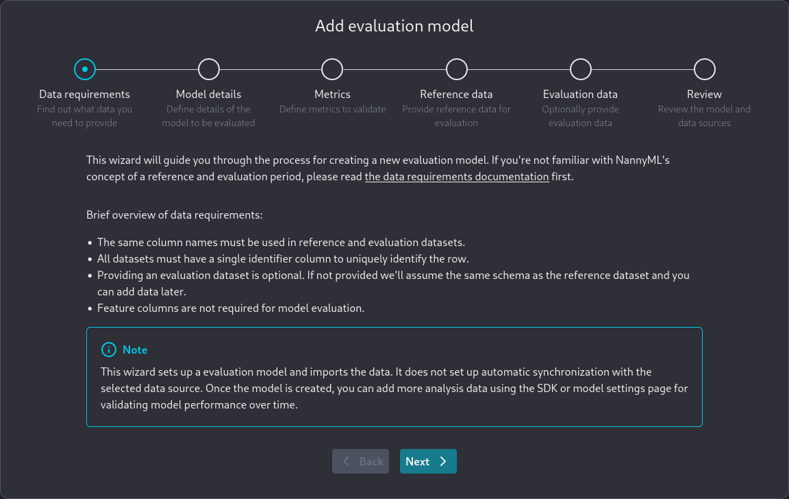
The first screen of the wizard shows some basic information needed to add a model.
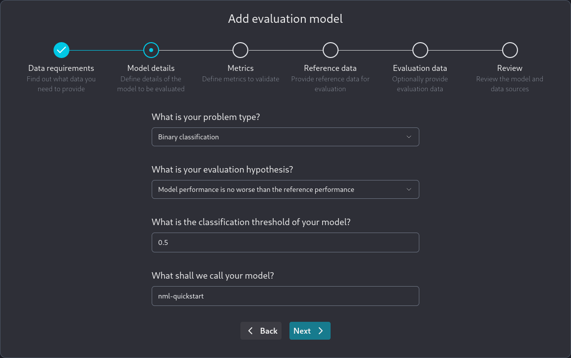
In the next screen you specify some important information about the model you are adding:
You need to specify:
The machine learning problem type of your model. Currently, only binary classification is supported.
What is your evaluation hypothesis? Available options are:
Model performance is no worse than reference performance
Model performance is within a specified range
What is the classification threshold of your model
The name of your model
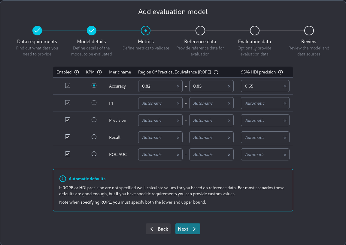
In the next screen, you need to define the metrics you want to validate.
ROPE and the required 95% HDI precision for each metric can be manually specified or inferred from the model's behavior on the reference data.
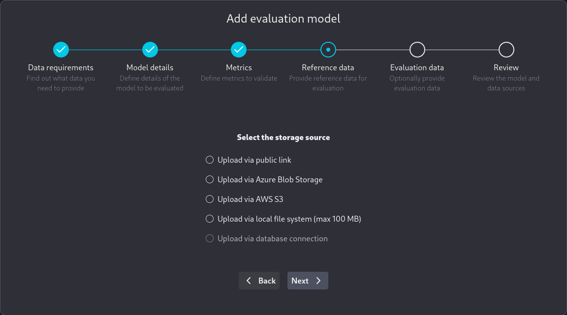
In the next screen, you are asked about specifying how you will provide your reference data.
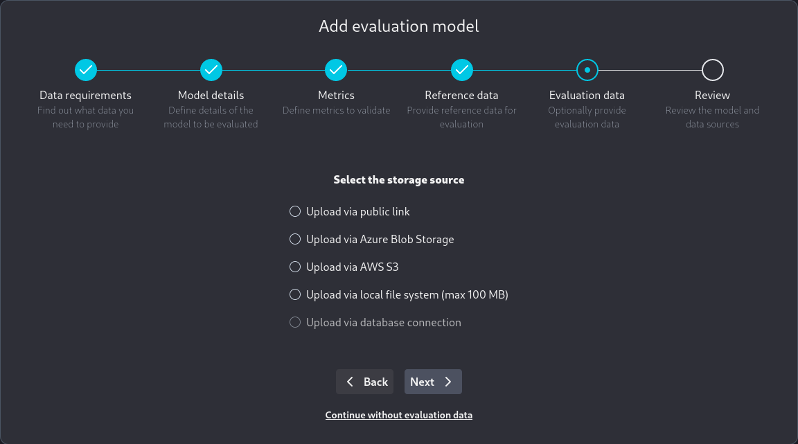
There are four options for adding new data—a public link, a local upload, and AWS S3 or Azure Blob storage.
We recommend using parquet files when uploading data using the user interface.
NannyML Cloud supports both parquet and CSV files, but CSV files don't store data type information. CSV files may cause incorrect data types to be inferred. If you later add more data to the model using the SDK or using parquet format, a data type conflict may occur.
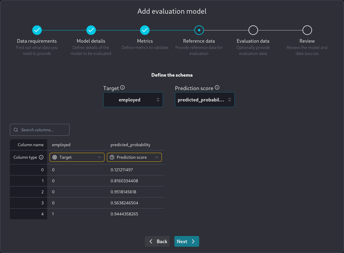
After providing your data, you need to specify what it contains, as seen below.
In the next screen, you are asked about specifying how you will provide your evaluation data.
This step is optional. If evaluation data is not currently available, it can be provided later.
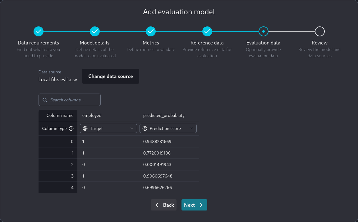
After providing the data we are again presented with a screen specifying their contents. Note that column names and data types cannot differ between reference and evaluation data.
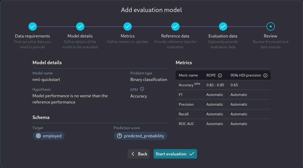
Finally, we have the review screen where we can review all the parameters we have specified regarding the new model:
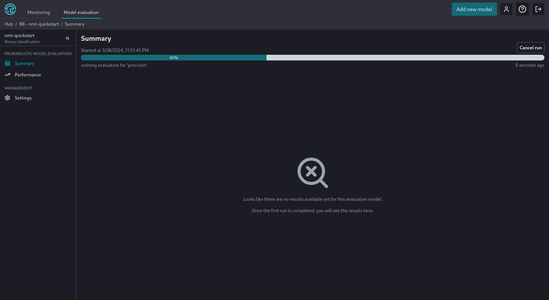
The application then goes to the model summary screen. If a run has not automatically started we can manually initiate it.
Adding more data
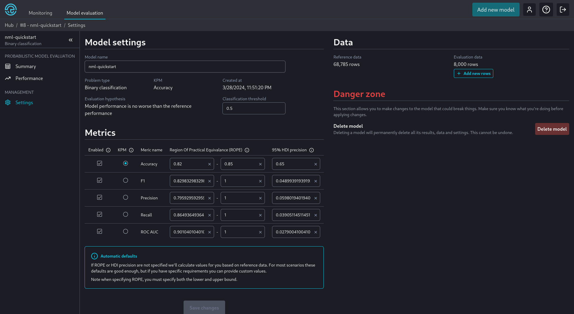
Quite often, we don't have all the data needed to evaluate a model immediately. When more data become available later, we can add them from the model settings screen. To do this we look at the Data section for the Add more rows button.
At this screen, we can also review the settings we chose during the model creation wizard and make any necessary changes.
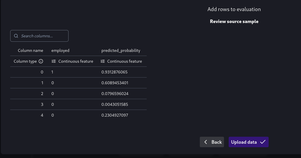
After we add more data, through a process similar to the one we used during the add model wizard, we are again presented with a confirmation screen.
Viewing Results
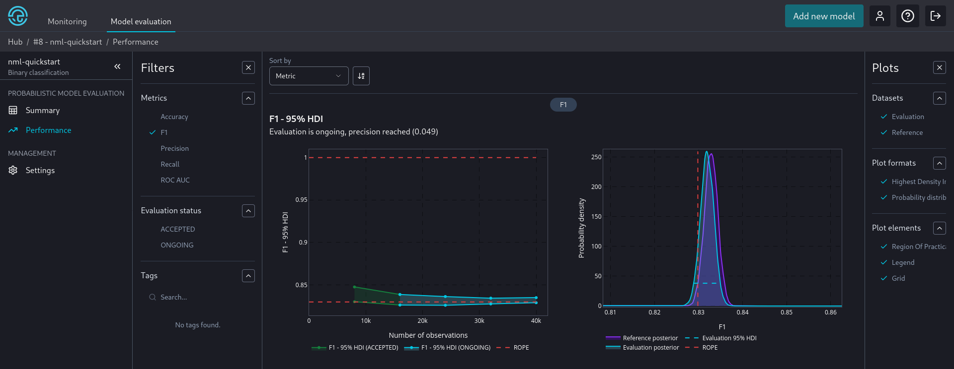
After we have added all available data and NannyML Cloud has finished processing them, we can view the results of the model evaluation. They are present in the Performance tab. We can see an example below:
We see that the F1 metric has been selected. There are two plots that show us how the model performs.
On the left, we see the evolution of the 95% HDI of the evaluated model as we add more observations. The limits of the ROPE area are shown as horizontal red dashed lines. The HDI is colored differently according to whether we have reached the required precision to make a decision and what that decision is.
On the right side we see the reference posterior and the latest evaluation posterior for F1. Again, the ROPE area limits are shown as vertical red dash lines.