Monitoring a computer vision model
The tutorial explaining how to monitor computer vision models with NannyML.
In this tutorial, we will use the model trained on the satellite image classification dataset that classifies the satellite image into one of the four classes: cloudy, desert, green area, and water. Later, we will show how to use NannyML to monitor the model performance with unseen production data. Additionally, we will show how to adapt the data drift detection methods for images.
The model and dataset
The dataset we will use is Satellite Image Classification Dataset-RSI-CB256 from Kaggle. The objective is to classify the satellite image into one of the four classes: cloudy, desert, green area, and water.
The dataset contains 5642 images, with 1500 images for water and green areas, 1510 for cloudy areas, and 1132 for dessert.
The production model is the ensemble of a pre-trained MobileNetV2 computer vision model used as a feature extractor, and the LGBM model is trained on the extracted features to classify the satellite image. The final model achieved 98% accuracy on the test set.
Reference and analysis sets
To evaluate the model in production, we have two sets:
Reference set - contains feature vector values extracted from the test set images along with the model’s predictions and labels. This set establishes a baseline for every metric we want to monitor.
Analysis set - contains feature vector values extracted from a production set with the model’s prediction, and in this case, labels. The analysis set is where NannyML analyzes/monitors the model’s performance and data drift of the model using the knowledge gained from the reference set.
Both sets contain features propagated through the model to get the predictions in tabular use cases. Since we’re dealing with images, our features represent the feature vector obtained from pre-trained MobileNetV2 architecture.
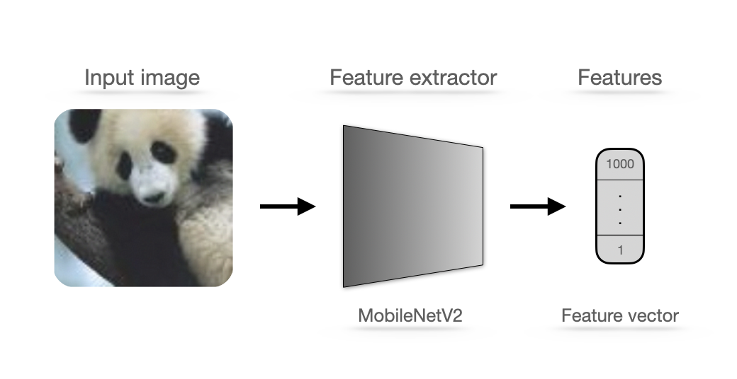
The resulting reference set and analysis set is a data frame with 1000 feature vector values(features), ground truth values, timestamp column, and model’s predictions for each class and predicted label and index column.
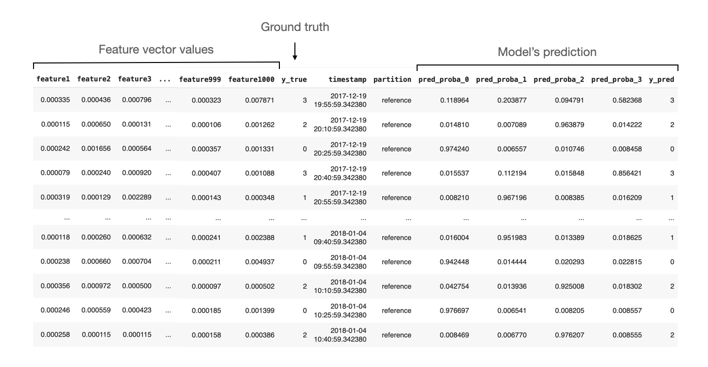
To upload the data to the nannyML cloud, use the Upload via public link option and use the following links:
Reference set -
https://github.com/NannyML/sample_datasets/blob/main/image_satellite/image_satellite_reference.pqAnalysis set -
https://github.com/NannyML/sample_datasets/blob/main/image_satellite/image_satellite_analysis.pq
Analyzing model performance in production
Once an ML model is in production, we would like to get a view of how the model is performing. The tricky part is that we can not always measure the realized performance. To calculate it, we need the correct targets, in this case, the labeled image. However, since images are usually manually labeled, it may take a while before they are updated to the system.
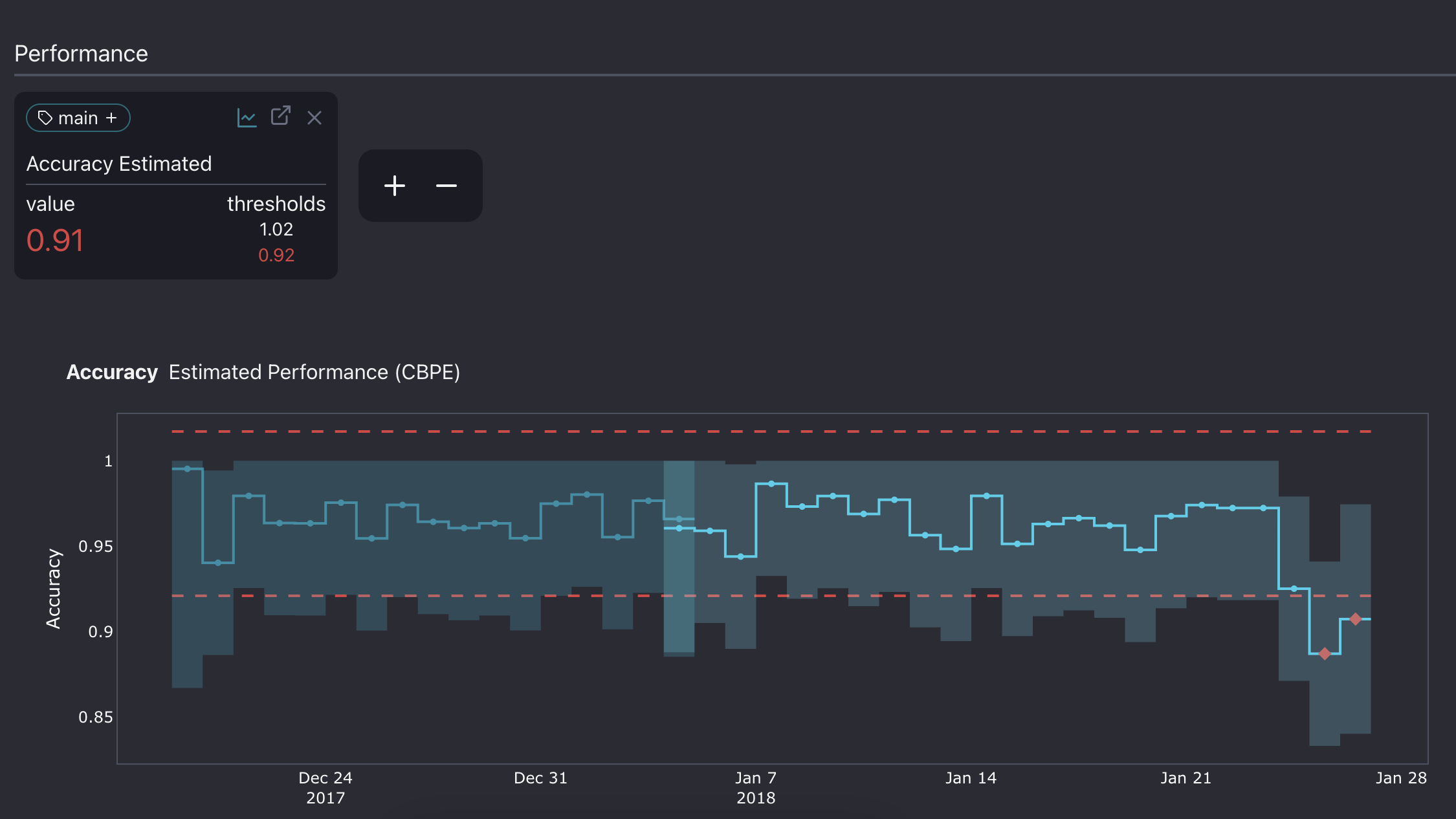
The plot above shows that the estimated performance exceeded the threshold during the last week of December, which means that the model failed to make reliable predictions during those days.
Comparing realized and estimated performance
When targets become available, we can calculate the realized performance on production data. It helps us better understand how the model behaved in production and evaluate NannyML estimations.
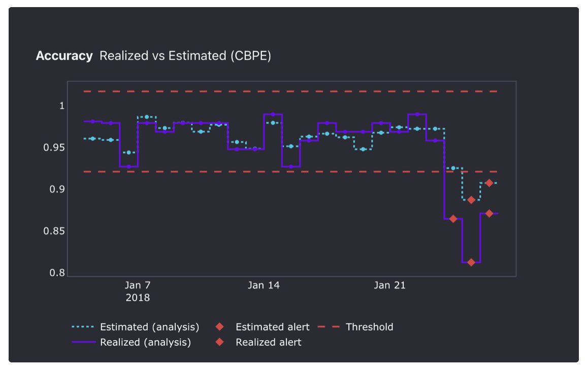
In the plot above, the estimated performance is usually close to the realized one, except for some points during the last two days. Performance degradation there is more significant than estimated.
The next step is to go down the rabbit hole and figure out what went wrong during those days.
We will use multivariate data drift detection methods to achieve this. It will allow us to check if a drift in the data caused the performance issue.
Detecting multivariate data drift
Multivariate data drift detection algorithm detects data drift by looking at any changes in the data structure.

It first compresses the reference feature space to a latent space using a PCA algorithm. The algorithm later decompresses the latent space data and reconstructs it with some error. This error is called the reconstruction error.
We can later use the learned compressor/decompressor to transform the production set and measure its reconstruction error. If the reconstruction error is larger than a threshold, the structure learned by PCA no longer accurately resembles the underlying structure of the analysis data. This indicates that there is data drift in the analysis/production data.
The method is designed for tabular(two-dimensional) data, but the image can also be compressed to that format using the pre-trained convolutional neural network as a feature extractor. The feature vector is an input to the multivariate drift algorithm, and based on it, the reconstruction error is calculated.
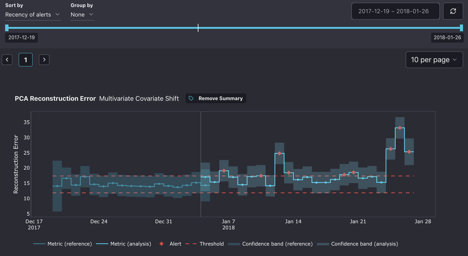
First, we notice quite a few false alerts in the drift detection. Also, on the 13th of January, a notable drift slightly affected the accuracy. In the last two days, there has also been a significant drift, which overlaps with the drop in performance.
Usually, we would need to inspect the individual images and look for any visual changes to find the reason behind the drift.
In our case, the last 200 images in our dataset have been augmented with an artificial drift that resembles the real one.
The common problem in cameras is chromatic aberration, where the colors on the images shift, caused by lens failure. As a result, "fringes" of color along boundaries separate dark and bright parts of the image(as you can see in the picture below).
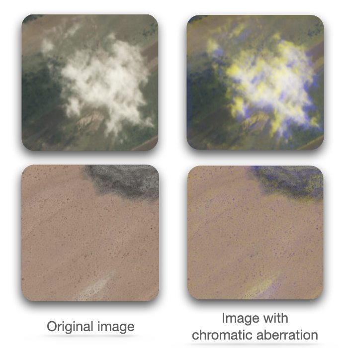
This is the reason behind the drop in the performance in the last two chunks and the spike in the reconstruction error.
Conclusions
We went through the monitoring workflow for the satellite image classification model. First, we started with data preparation and performance estimation. Then, we evaluated the estimated performance with the realized performance estimation and confirmed the significant drop in the last two chunks. Later, we used a multivariate drift detection method to determine if the data drift was responsible.