NannyML Cloud
HomeBlogNannyML OSS Docs
v0.23.0
v0.23.0
  • ☂️Introduction
  • Model Monitoring
    • Quickstart
    • Data Preparation
      • How to get data ready for NannyML
    • Tutorials
      • Monitoring a tabular data model
      • Monitoring with segmentation
      • Monitoring a text classification model
      • Monitoring a computer vision model
    • How it works
      • Probabilistic Adaptive Performance Estimation (PAPE)
      • Reverse Concept Drift (RCD)
    • Custom Metrics
      • Creating Custom Metrics
        • Writing Functions for Binary Classification
        • Writing Functions for Multiclass Classification
        • Writing Functions for Regression
        • Handling Missing Values
        • Advanced Tutorial: Creating a MTBF Custom Metric
      • Adding a Custom Metric through NannyML SDK
  • Product tour
    • Navigation
    • Adding a model
    • Model overview
    • Deleting a model
    • Model side panel
      • Summary
      • Performance
      • Concept drift
      • Covariate shift
      • Data quality
      • Logs
      • Model settings
        • General
        • Data
        • Performance settings
        • Concept Drift settings
        • Covariate Shift settings
        • Descriptive Statistics settings
        • Data Quality settings
    • Account settings
  • Deployment
    • Azure
      • Azure Managed Application
        • Finding the URL to access managed NannyML Cloud
        • Enabling access to storage
      • Azure Software-as-a-Service (SaaS)
    • AWS
      • AMI with CFT
        • Architecture
      • EKS
        • Quick start cluster setup
      • S3 Access
    • Application setup
      • Authentication
      • Notifications
      • Webhooks
      • Permissions
  • NannyML Cloud SDK
    • Getting Started
    • API Reference
  • Probabilistic Model Evaluation
    • Introduction
    • Tutorials
      • Evaluating a binary classification model
      • Data Preparation
    • How it works
      • HDI+ROPE (with minimum precision)
      • Getting Probability Distribution of a Performance Metric with targets
      • Getting Probability Distribution of Performance Metric without targets
      • Getting Probability Distribution of Performance Metric when some observations have labels
      • Defaults for ROPE and estimation precision
  • Experiments Module
    • Introduction
    • Tutorials
      • Running an A/B test
      • Data Preparation
    • How it works
      • Getting probability distribution of the difference of binary downstream metrics
  • miscellaneous
    • Engineering
    • Usage logging in NannyNL
    • Versions
      • Version 0.23.0
      • Version 0.22.0
      • Version 0.21.0
Powered by GitBook
On this page
  • Introducing Custom Metrics
  • Using Custom Metrics
  1. Model Monitoring

Custom Metrics

Monitoring Models with Custom Metrics

PreviousReverse Concept Drift (RCD)NextCreating Custom Metrics

Introducing Custom Metrics

NannyML offers some standard metrics to monitor your classification and regression models. But sometimes you need something more customized to ensure your model performs adequately. The Custom Metrics functionality solves this issue. You can create custom metrics to monitor your machine learning models in ways better suited to your particular circumstances.

NannyML allows you to both calculate the performance of your model using your custom metric but also estimate the performance according to that custom metric. Let's see how this works!

Using Custom Metrics

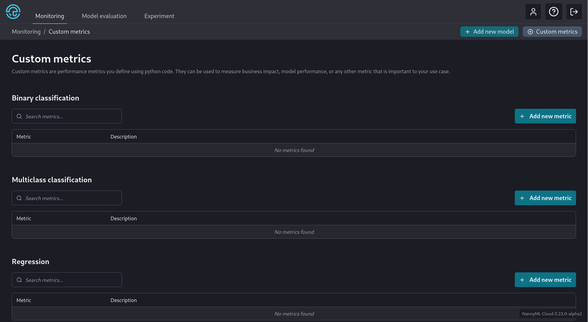
You can access the Custom Metrics settings on the top left of your screen, as you can see below:

There are three types of custom metrics supported. Binary Classification, Multiclass Classification, and Regression. They are organized separately on the Custom Metrics settings page shown below:

It is straightforward to add a new custom metric. Let's go through the process for each metric type.

We click the appropriate Add new metric button as seen below:

We are then greeted with a new screen where we have to enter the information related to the new metric:

As shown we need to fill in the following information:

  • A name for the metric.

  • A short description of the metric.

  • A function that calculates the metric.

  • A function that estimates the metric

  • The numerical limits of the metric, if they exist.

import numpy as np
import pandas as pd
from sklearn.metrics import fbeta_score

def calculate(
    y_true: pd.Series,
    y_pred: pd.Series,
    y_pred_proba: pd.DataFrame,
    chunk_data: pd.DataFrame,
    labels: list[str],
    class_probability_columns: list[str],
    **kwargs
) -> float:
    # labels and class_probability_columns are only needed for multiclass classification
    # and can be ignored for binary classification custom metrics
    return fbeta_score(y_true, y_pred, beta=2)

while the required estimation function is:

import numpy as np
import pandas as pd

def estimate(
    estimated_target_probabilities: pd.DataFrame,
    y_pred: pd.Series,
    y_pred_proba: pd.DataFrame,
    chunk_data: pd.DataFrame,
    labels: list[str],
    class_probability_columns: list[str],
    **kwargs
) -> float:
    # labels and class_probability_columns are only needed for multiclass classification
    # and can be ignored for binary classification custom metrics

    estimated_target_probabilities = estimated_target_probabilities.to_numpy().ravel()
    y_pred = y_pred.to_numpy()

    # Create estimated confusion matrix elements
    est_tp = np.sum(np.where(y_pred == 1, estimated_target_probabilities, 0))
    est_fp = np.sum(np.where(y_pred == 1, 1 - estimated_target_probabilities, 0))
    est_fn = np.sum(np.where(y_pred == 0, estimated_target_probabilities, 0))
    est_tn = np.sum(np.where(y_pred == 0, 1 - estimated_target_probabilities, 0))

    beta = 2
    fbeta =  (1 + beta**2) * est_tp / ( (1 + beta**2) * est_tp + est_fp + beta**2 * est_fn)
    fbeta = np.nan_to_num(fbeta)
    return fbeta

The default metric limits still apply, so we can leave those as they are. These metric limits ensure that the metric thresholds are constrained to these theoretical limits. We then fill all this information on the new binary classification metric screen:

This results in the new metric now being visible in the Binary Classification section of the Custom Metrics screen.

The metric can now be selected for use by any binary classification model from the Model Settings page.

We click the appropriate Add new metric button as seen below:

We are then greeted with a new screen where we have to enter the information related to the new metric:

As shown we need to fill in the following information:

  • A name for the metric.

  • A short description of the metric.

  • A function that calculates the metric.

  • A function that estimates the metric

  • The numerical limits of the metric, if they exist.

import pandas as pd
from sklearn.metrics import fbeta_score

def calculate(
    y_true: pd.Series,
    y_pred: pd.Series,
    y_pred_proba: pd.DataFrame,
    chunk_data: pd.DataFrame,
    labels: list[str],
    class_probability_columns: list[str],
) -> float:
    return fbeta_score(y_true, y_pred, beta=2, average='macro')

while the required estimate function is:

import numpy as np
import pandas as pd
from sklearn.preprocessing import label_binarize

def estimate(
    estimated_target_probabilities: pd.DataFrame,
    y_pred: pd.Series,
    y_pred_proba: pd.DataFrame,
    chunk_data: pd.DataFrame,
    labels: list[str],
    class_probability_columns: list[str],
):
    beta = 2

    def estimate_fb(_y_pred, _y_pred_proba, beta) -> float:
        # Estimates the Fb metric.
        #
        # Parameters
        # ----------
        # y_pred: np.ndarray
        #     Predicted class label of the sample
        # y_pred_proba: np.ndarray
        #     Probability estimates of the sample for each class in the model.
        # beta: float
        #     beta parameter
        #
        # Returns
        # -------
        # metric: float
        #     Estimated Fb score.
        

        est_tp = np.sum(np.where(_y_pred == 1, _y_pred_proba, 0))
        est_fp = np.sum(np.where(_y_pred == 1, 1 - _y_pred_proba, 0))
        est_fn = np.sum(np.where(_y_pred == 0, _y_pred_proba, 0))
        est_tn = np.sum(np.where(_y_pred == 0, 1 - _y_pred_proba, 0))

        fbeta =  (1 + beta**2) * est_tp / ( (1 + beta**2) * est_tp + est_fp + beta**2 * est_fn)
        fbeta = np.nan_to_num(fbeta)
        return fbeta

    estimated_target_probabilities = estimated_target_probabilities.to_numpy()
    y_preds = label_binarize(y_pred, classes=labels)

    ovr_estimates = []
    for idx, _  in enumerate(labels):
        ovr_estimates.append(
            estimate_fb(
                y_preds[:, idx],
                estimated_target_probabilities[:, idx],
                beta=2
            )
        )
    multiclass_metric = np.mean(ovr_estimates)

    return multiclass_metric

The default metric limits still apply, so we can leave those as they are. These metric limits ensure that the metric thresholds are constrained to these theoretical limits.

We then fill all this information on the new multiclass classification metric screen:

This results in the new metric now being visible in the Binary Classification section of the Custom Metrics screen.

The metric can now be selected for use by any multiclass classification model from the Model Settings page.

We click the appropriate Add new metric button as seen below:

We are then greeted with a new screen where we have to enter the information related to the new metric:

As shown we need to fill in the following information:

  • A name for the metric.

  • A short description of the metric.

  • A function that calculates the loss of the metric.

  • A function that aggregates the loss results in order to calculate the metric

  • The numerical limits of the metric, if they exist.

import numpy as np
import pandas as pd

def loss(
    y_true: pd.Series,
    y_pred: pd.Series,
    chunk_data: pd.DataFrame,
    **kwargs
) -> np.ndarray:
    y_true = y_true.to_numpy()
    y_pred = y_pred.to_numpy()

    alpha = 0.9
    factor1 = alpha * np.maximum(y_true - y_pred, 0)
    factor2 = (1 - alpha) * np.maximum(y_pred - y_true, 0)
    return factor1 + factor2

while the required aggregate function is:

import numpy as np
import pandas as pd

def aggregate(
    loss: np.ndarray,
    chunk_data: pd.DataFrame,
    **kwargs
) -> float:
    return loss.mean()

The default metric limits still apply, so we can leave those as they are. These metric limits ensure that the metric thresholds are constrained to these theoretical limits.

We then fill all this information on the new regression metric screen:

This results in the new metric now being visible in the Regression section of the Custom Metrics screen.

The metric can now be selected for use by any regression model from the Model Settings page.

Note that once custom metrics are added they can be selected during the Add new model wizard. You can see the relevant step for binary classification in the screenshot below:

Custom metrics can also be selected from a model's settings page

Developing the code for the required functions is described for the f_beta score. The required calculation function is:

Developing the code for the required functions is described for the f_beta score. The required calculate function is:

Developing the code for the required functions is described for the pinball score. The required loss function is:

here
here
here
Accessing the Custom Metrics Settings
Custom Settings screen
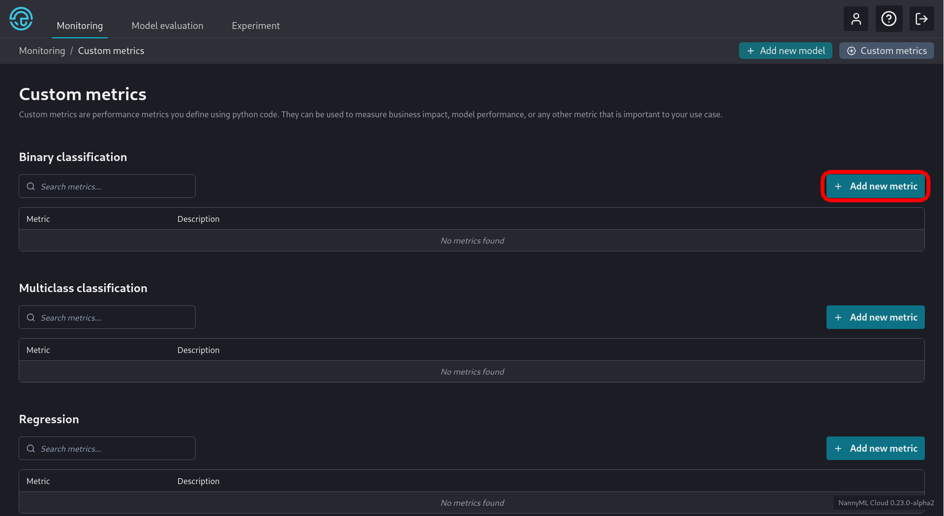
Adding a new Custom Binary Classification Metric
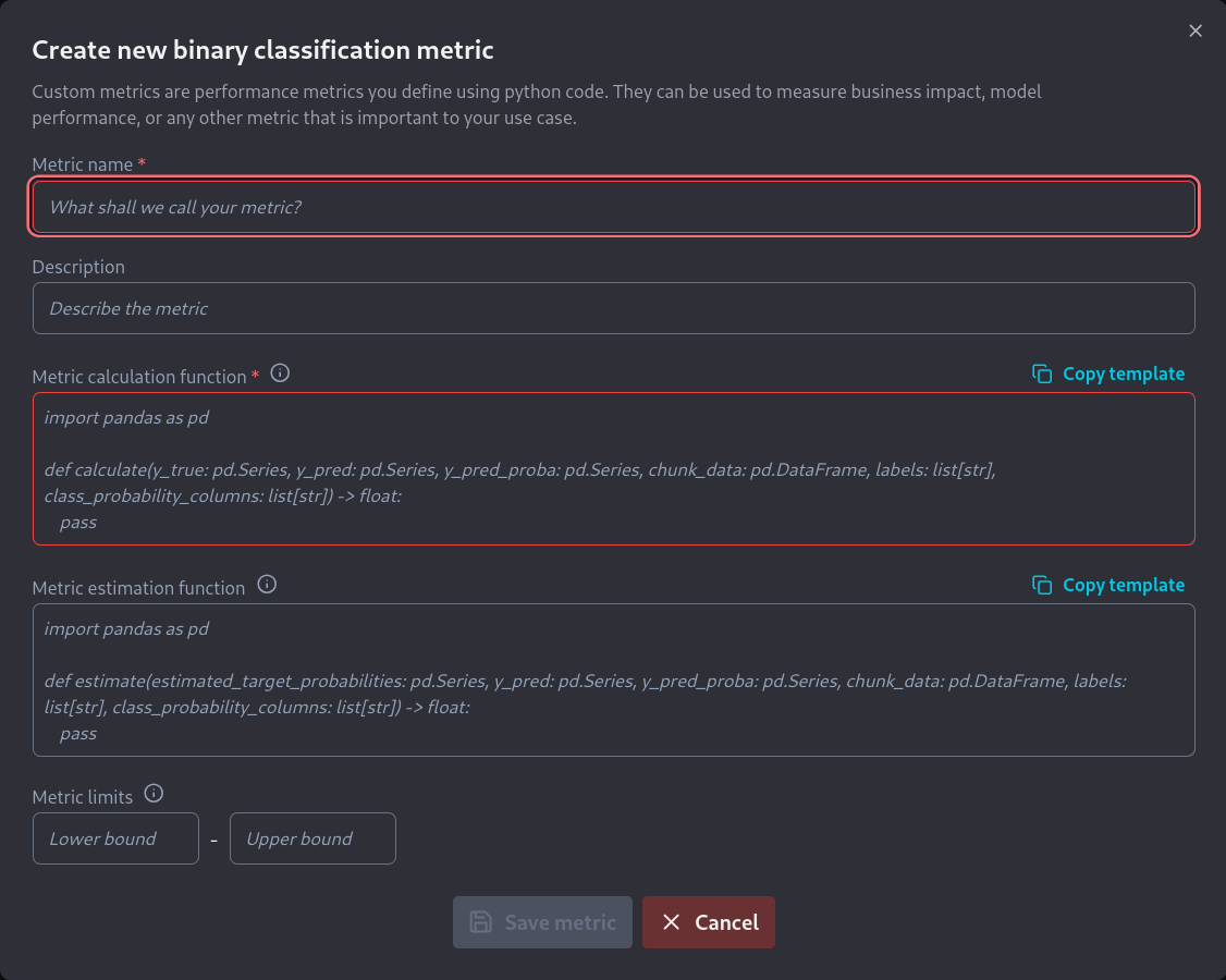
New Custom Binary Classification Metric screen
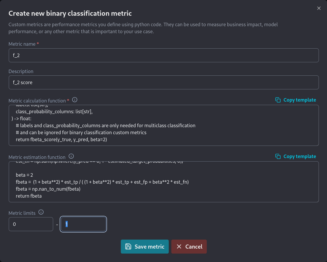
Completing the new binary classification metric screen
f_2 binary classification metric
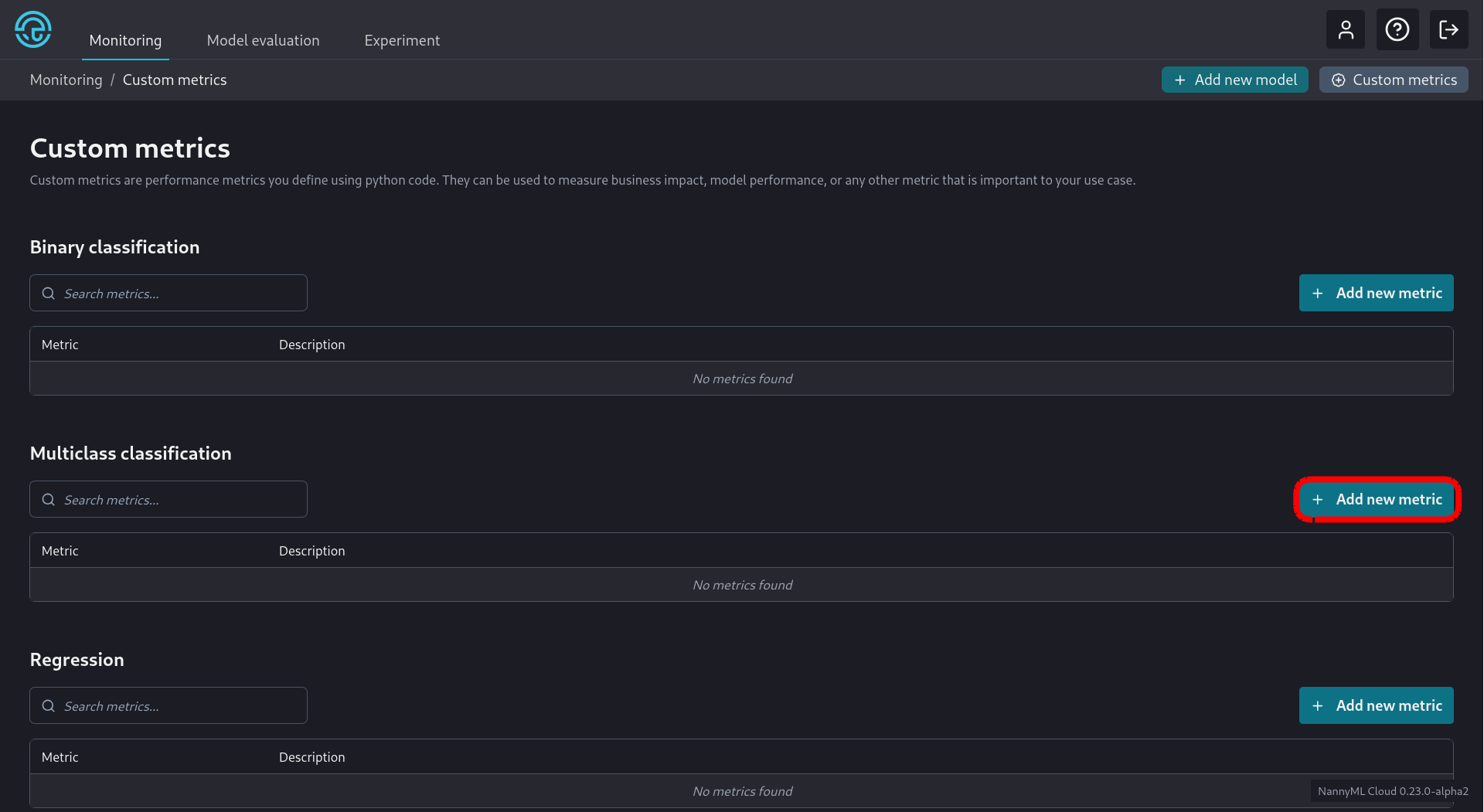
Adding a new Custom Multiclass Classification Metric
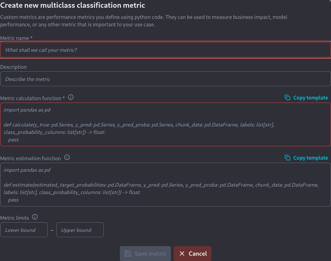
New Custom Multiclass Classification Metric screen
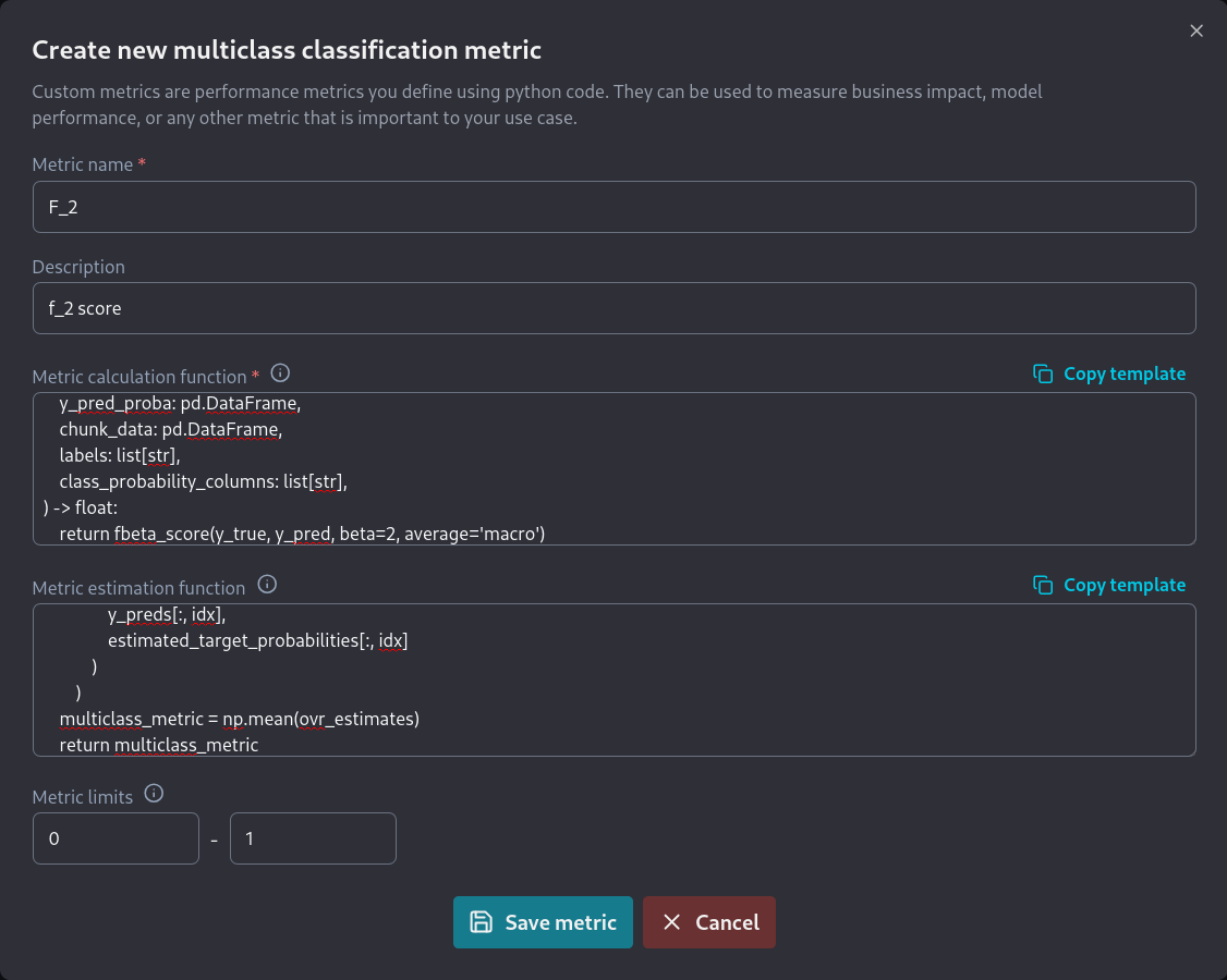
Completing the new multiclass classification metric screen
F_2 multiclass classification metric
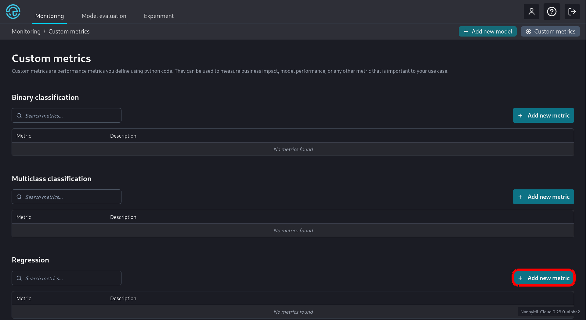
Adding a new Custom Regression Metric
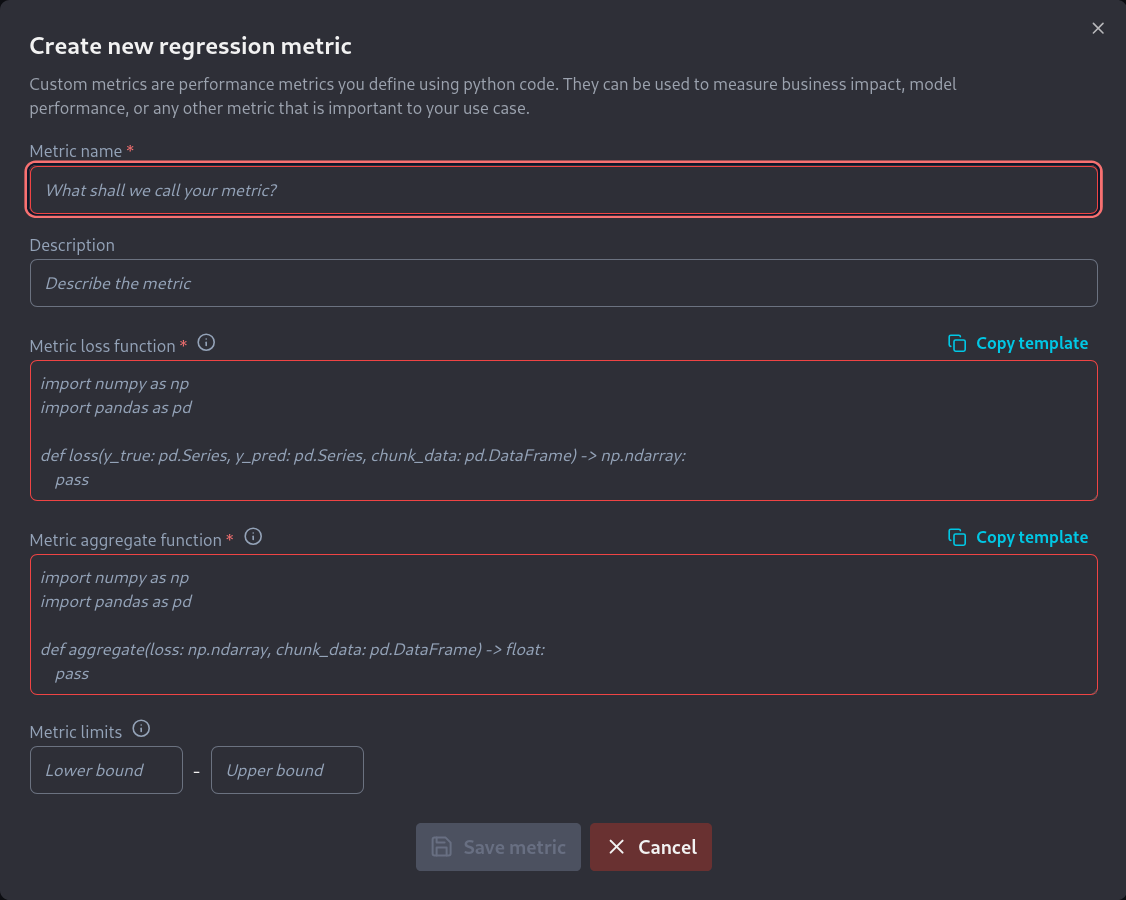
New Custom Regression Metric screen
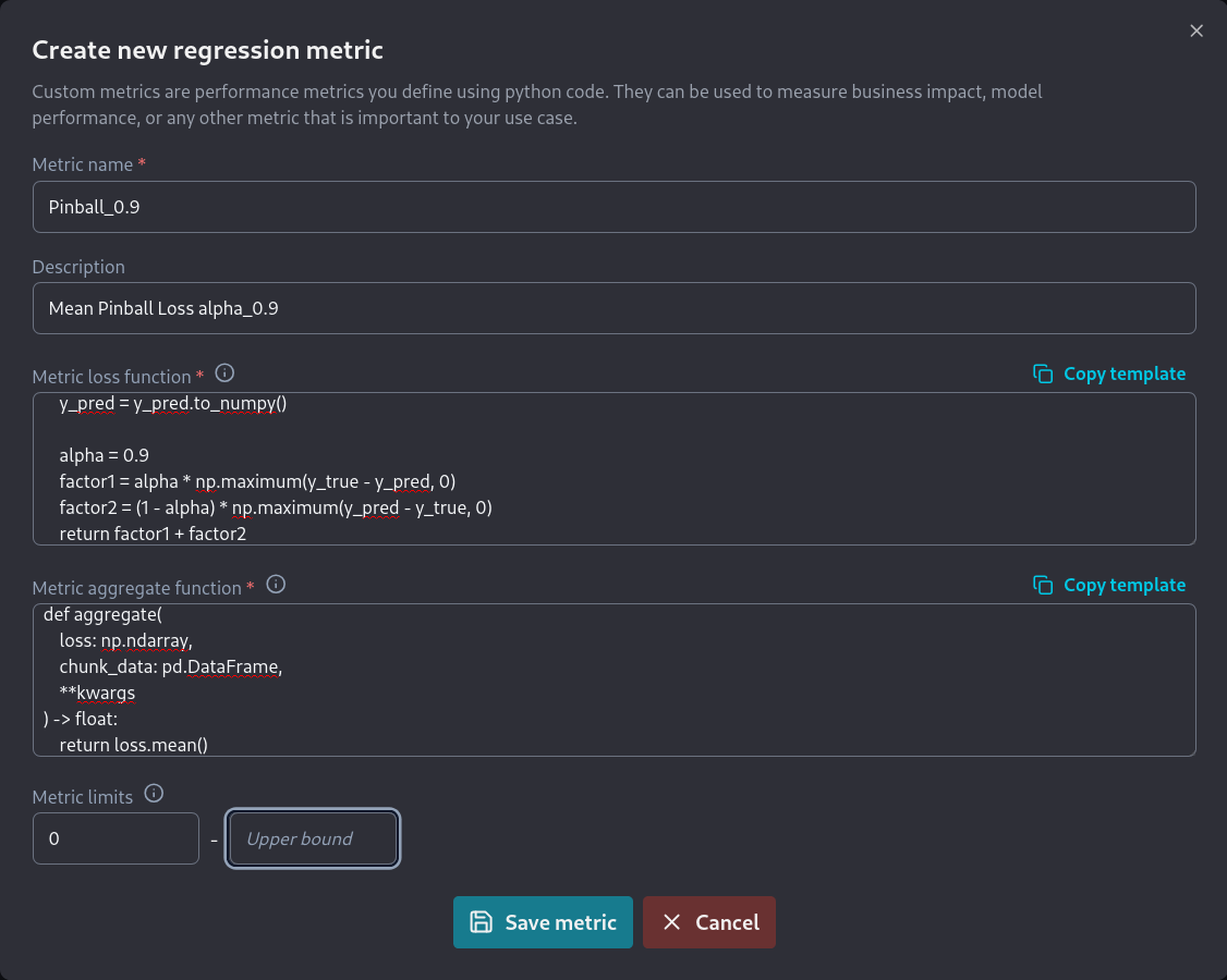
Completing the new regression metric screen
F_2 multiclass classification metric
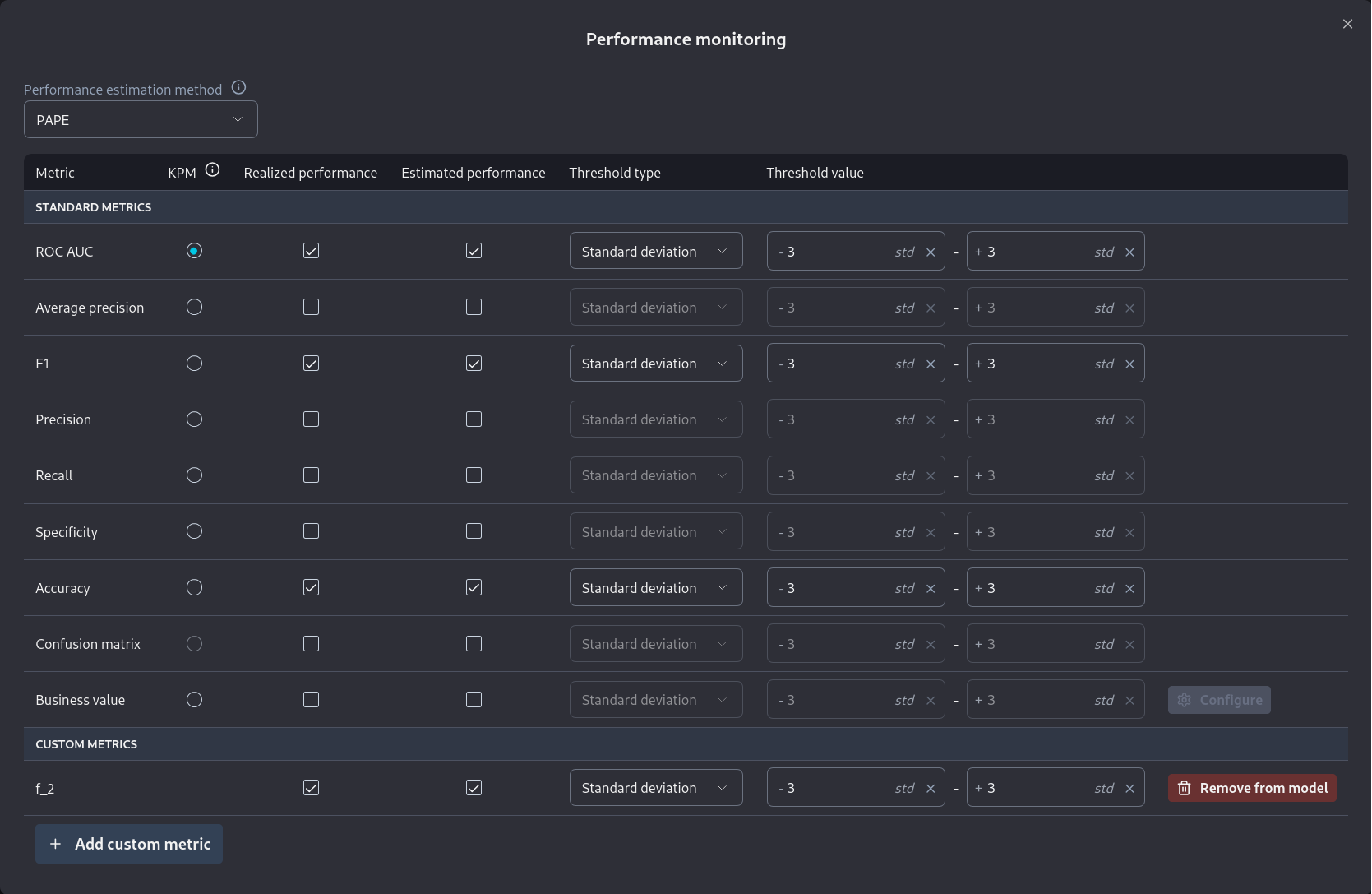
Enabling a custom metric during the Add new model wizard.
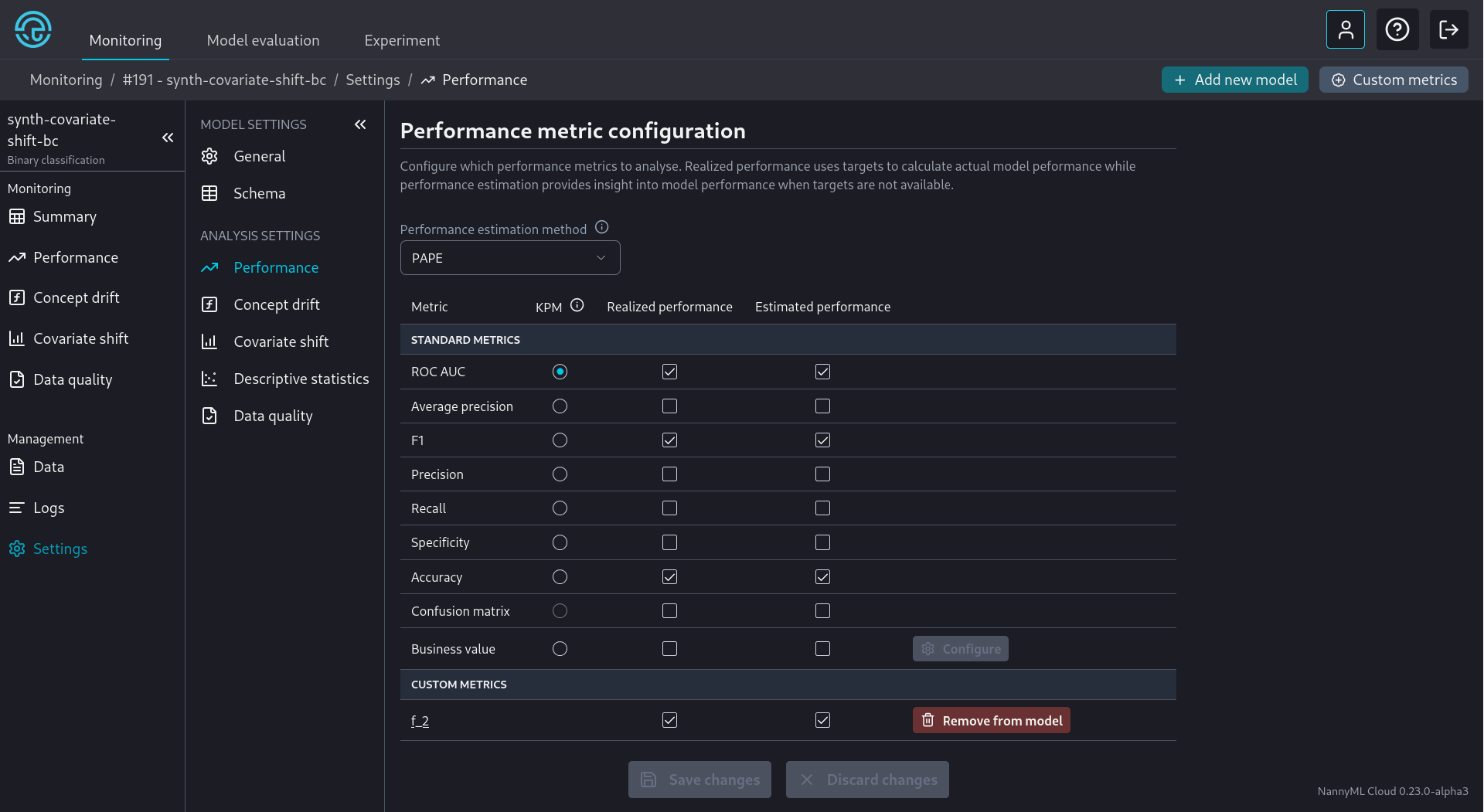
Selecting Custom Metrics from a model's Performance Settings