Advanced Tutorial: Creating a MTBF Custom Metric

Creating a MTBF custom metric using the timestamp column from chunk data.

Often we will need to create more complicated custom metrics. Let's use Mean Time Between Failures as an example. In order to calculate it we will need information from columns in the chunk data dataframe.

We will assume the user has access to a Jupyter Notebook running Python with the NannyML open-source library installed.

Repurposing our binary classification sample dataset

We will be using the same dataset we saw when writing custom metric functions for binary classification. The dataset is publicly accessible here. It is a pure covariate shift dataset that consists of:

  • 5 numerical features: ['feature1', 'feature2', 'feature3', 'feature4', 'feature5',]

  • Target column: y_true

  • Model prediction column: y_pred

  • The model predicted probability: y_pred_proba

  • A timestamp column: timestamp

  • An identifier column: identifier

  • The probabilities from which the target values have been sampled: estimated_target_probabilities

Here the meaning of the dataset will be a little different. We have some machines operating over a time period. We are also performing regular checks on them to see if there are any failures. We can aggregate our results over this time period to see how many failures we observed over that period compared to the total operating time of all machines inspected during this period. This will be our simple MTBF metric.

We can inspect the dataset with the following code in a Jupyter cell:

import pandas as pd
import nannyml as nml

reference = pd.read_parquet("https://github.com/NannyML/sample_datasets/raw/main/synthetic_pure_covariate_shift_datasets/binary_classification/synthetic_custom_metrics_binary_classification_reference.pq")
monitored = pd.read_parquet("https://github.com/NannyML/sample_datasets/raw/main/synthetic_pure_covariate_shift_datasets/binary_classification/synthetic_custom_metrics_binary_classification_monitored.pq")
reference.head(5)
+----+------------+------------+------------+------------+------------+----------+----------------+----------+----------------------------+--------------+----------------------------------+
|    | feature1   | feature2   | feature3   | feature4   | feature5   | y_true   | y_pred_proba   | y_pred   | timestamp                  | identifier   | estimated_target_probabilities   |
+====+============+============+============+============+============+==========+================+==========+============================+==============+==================================+
| 0  | 0.507982   | 2.10996    | -3.29121   | 2.59278    | 0.970656   | 0        | 0.0208479      | 0        | 2020-03-25 00:00:00        | 60000        | 0.0218986                        |
+----+------------+------------+------------+------------+------------+----------+----------------+----------+----------------------------+--------------+----------------------------------+
| 1  | -3.21001   | 2.27251    | -0.0506065 | 0.641354   | 1.82951    | 1        | 0.960223       | 1        | 2020-03-25 00:02:00.960000 | 60001        | 0.959278                         |
+----+------------+------------+------------+------------+------------+----------+----------------+----------+----------------------------+--------------+----------------------------------+
| 2  | -0.135355  | 1.13828    | -0.106979  | 0.642139   | -0.647236  | 1        | 0.502806       | 1        | 2020-03-25 00:04:01.920000 | 60002        | 0.507093                         |
+----+------------+------------+------------+------------+------------+----------+----------------+----------+----------------------------+--------------+----------------------------------+
| 3  | -2.35321   | -1.0053    | -1.05535   | 1.64436    | 0.251892   | 1        | 0.784257       | 1        | 2020-03-25 00:06:02.880000 | 60003        | 0.785474                         |
+----+------------+------------+------------+------------+------------+----------+----------------+----------+----------------------------+--------------+----------------------------------+
| 4  | 0.667785   | 1.38383    | -1.28428   | -0.0995213 | -1.21584   | 0        | 0.121911       | 0        | 2020-03-25 00:08:03.840000 | 60004        | 0.124328                         |
+----+------------+------------+------------+------------+------------+----------+----------------+----------+----------------------------+--------------+----------------------------------+

Developing the MTBF metric functions

NannyML Cloud requires two functions for the custom metric to be used. The first is the calculate function, which is mandatory, and is used to calculate realized performance for the custom metric. The second is the estimate function, which is optional, and is used to do performance estimation for the custom metric when target values are not available.

To create a custom metric from the MTBF metric we create the calculate function below:

import pandas as pd

def calculate(
    y_true: pd.Series,
    y_pred: pd.Series,
    y_pred_proba: pd.DataFrame,
    chunk_data: pd.DataFrame,
    **kwargs
) -> float:
    _max = chunk_data['timestamp'].max()
    _min = chunk_data['timestamp'].min()
    hours = len(y_true) * (_max - _min).seconds / 3600
    failures = y_true.sum()
    return hours/failures

The estimate function is relatively straightforward in our case. We can estimate the number of failures by using the sum of estimated_target_probabilities. Hence we get:

import pandas as pd

def estimate(
    estimated_target_probabilities: pd.DataFrame,
    y_pred: pd.Series,
    y_pred_proba: pd.DataFrame,
    chunk_data: pd.DataFrame,
    **kwargs
) -> float:
    _max = chunk_data['timestamp'].max()
    _min = chunk_data['timestamp'].min()
    hours = len(y_pred) * (_max - _min).seconds / 3600
    failures = estimated_target_probabilities.sum()
    return (hours/failures)[0]

We can test those functions on the dataset loaded earlier. Assuming we run the functions as provided in a Jupyter cell we can then call them. Running calculate we get:

class_probability_columns = ['y_pred_proba',]
labels = [0, 1]

estimate(
    reference[['estimated_target_probabilities']],
    reference['y_pred'],
    reference[class_probability_columns],
    reference,
    labels=labels,
    class_probability_columns=class_probability_columns
)
47.75475389197522

While running estimate we get:

calculate(
    reference['y_true'],
    reference['y_pred'],
    reference[class_probability_columns],
    reference,
    labels=labels,
    class_probability_columns=class_probability_columns
)
47.57281018074348

We can see that the values between estimated and realized MTBF score are very close. This means that we are likely estimating the metric correctly. The values will never match due to the statistical nature of the problem. Sampling error will always induce some differences.

Testing MTBF in the Cloud product

We saw how to add a binary classification custom metric in the Custom Metrics Introductory page. We can further test it by using the dataset in the cloud product. The datasets are publically available hence we can use the Public Link option when adding data to a new model.

Reference Dataset Public Link:

https://github.com/NannyML/sample_datasets/raw/main/synthetic_pure_covariate_shift_datasets/binary_classification/synthetic_custom_metrics_binary_classification_reference.pq

Monitored Dataset Public Link:

https://github.com/NannyML/sample_datasets/raw/main/synthetic_pure_covariate_shift_datasets/binary_classification/synthetic_custom_metrics_binary_classification_monitored.pq

The process of creating a new model is described in the Monitoring a tabular data model.

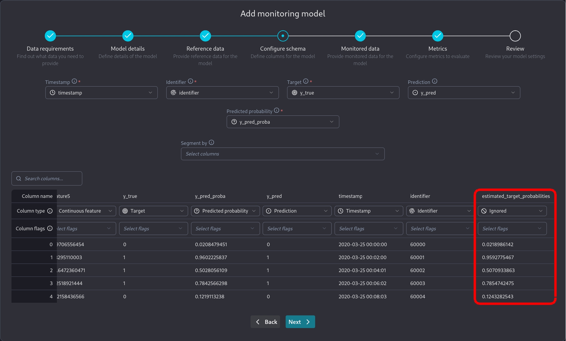
We need to be careful to mark estimated_target_probabilities as an ignored column since it's related to our oracle knowledge of the problem and not to the monitored model the dataset represents.

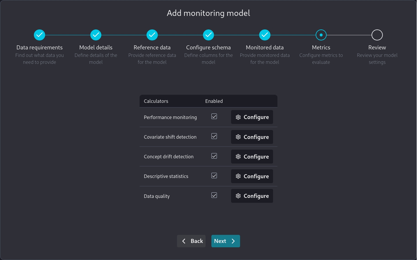
Note that when we are on the Metrics page

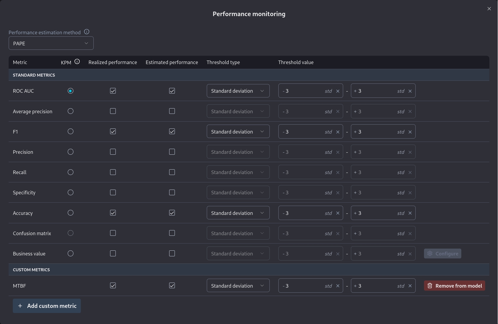
we can go to Performance monitoring and directly add a custom metric we have already specified.

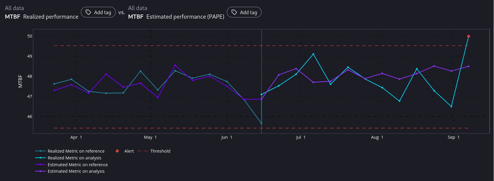
After the model has been added to NannyML Cloud and the first run has been completed we can inspect the monitoring results. Of particular interest to us is the comparison between estimated and realized performance for our custom metric.

We see that NannyML can accurately estimate our custom metric across the whole dataset. Even in the areas where there is a performance difference. This means that our calculate and estimate functions have been correctly created as the dataset is created specifically to facilitate this test.

You may have noticed that for custom metrics we don't have a sampling error implementation. Therefore you will have to make a qualitative judgement, based on the results, whether the estimated and realized performance results are a good enough match or not.

Next Steps

You are now ready to use your new custom metric in production. However, you may want to make your implementation more robust to account for the data you will encounter in production. For example, you can add missing value handling to your implementation.