Getting Probability Distribution of Performance Metric without targets

This page describes how NannyML estimates the probability distribution of a performance metric when targets are not available.

As described in the Introduction, Probabilistic Model Evaluation uses performance metric probability distribution estimated with the Bayesian approach. This is particularly difficult when the targets are not available. The high-level overview of the solution is described below. It assumes basic familiarity with .

The intuition

When the targets are available, the Bayesian posterior of a probability metric quantifies all sources of uncertainty. The prediction and its evaluation can be considered as a two-step random process. First, we draw from the population of inputs. We then use the ML model to get a prediction from these inputs. Then, we draw from the conditional probability of observing the target (given the inputs). The following example should clarify: consider a simple model that estimates whether an individual will repay the loan based on one binary feature only - that feature tells whether an individual is an entrepreneur or an employee. Now, assume that the probability of repaying the loan for an employee is 90 %, while for the entrepreneur is 75 %. So, the model returns the binary prediction of 1 (that it will be repaid) for both cases and the respective probabilities. The fact that the model always returns a binary prediction of 1 does not make it very useful in the real world, but it simplifies things for our example. Now, we are interested in the accuracy of our model (that is, whether prediction 1 is correct). So, the two sources of uncertainty are the following:

1. What is the type of the loan applicant (employer vs entrepreneur). This is drawing from inputs based on their probability distribution.

2. Given the type of result in step 1, we have a conditional probability of repaying the loan. We wait and see what the reality brings (whether it will be repaid). This draws from targets based on the probability of observing a positive target.

Now, there is no step 2 when the labels are unavailable. If the predicted probabilities returned by the model are the true conditional probabilities (or, in other words, if the model is perfectly calibrated), the model's accuracy depends only on step 1. That may sound counterintuitive, but when working on calibrated probabilities, the posterior of estimated performance is more precise (that is - the HDI width is smaller) compared to the situation with labels for the same amount of data. That sounds like having less information (no targets) gives you more information (more precise posterior estimation). It is the calibrated probabilities assumption that makes the difference. Having calibrated probabilities is more powerful than just observing which targets are drawn. Think about a coin whose (calibrated) probability of landing heads is 0.5. Compare it to observing that a coin lands heads five times out of ten. The former information tells you without uncertainty that the coin is fair. The latter does not. The 2nd step of the random process of evaluating a model described above is just like tossing this coin. We don't have to do it if we already have calibrated probability. Consider the following extreme: we only have one type of candidate - an entrepreneur - and we know that the probability is calibrated. The accuracy score is exactly equal to the probability of repayment for this type of candidate (that is 0.75) with no uncertainty at all. The posterior of accuracy is a single value - 0.75 - with 100% probability. Having calibrated probabilities removed step-2-related uncertainty while limiting the possible input value to only remove the uncertainty from step 1.

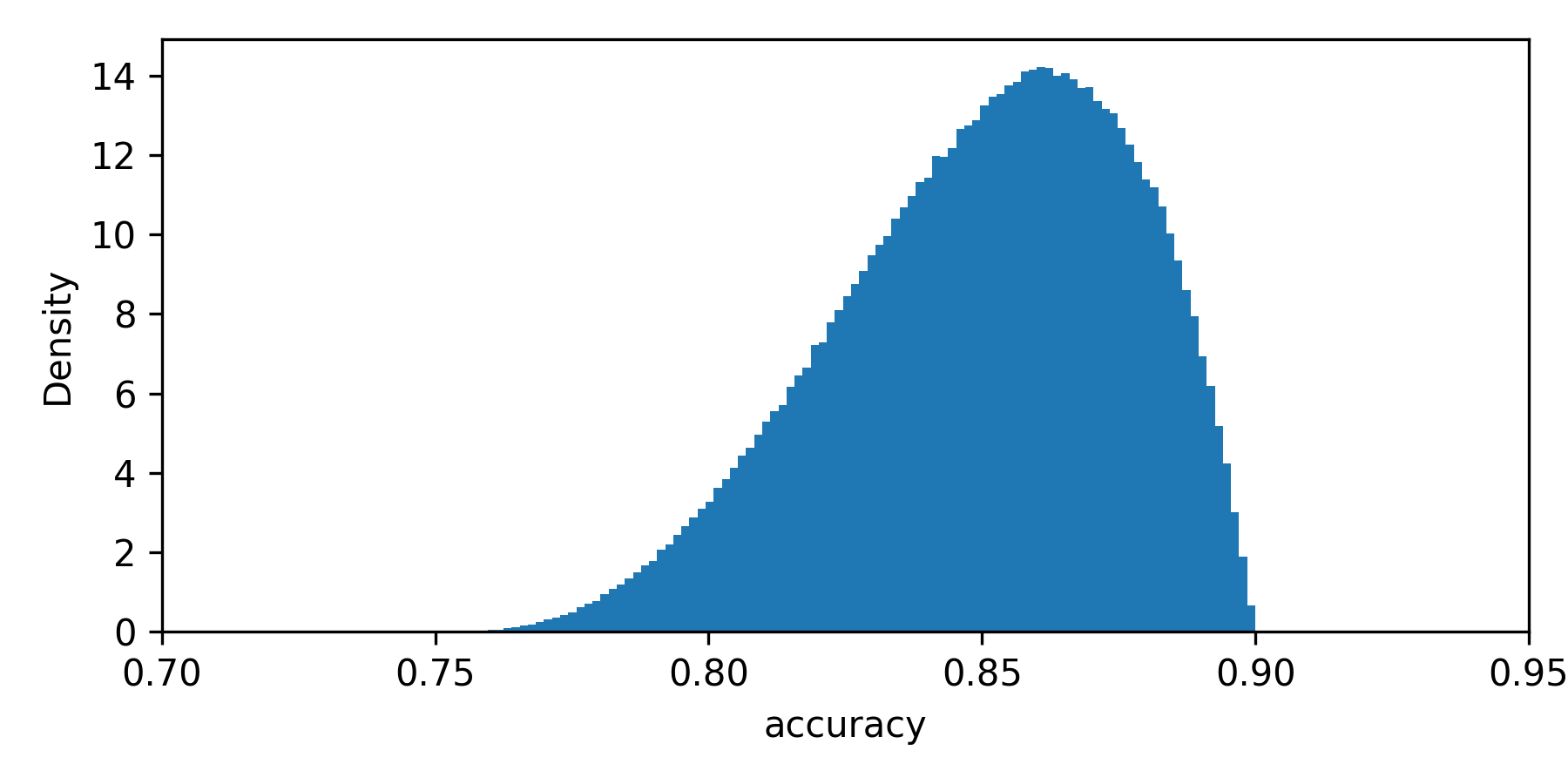
Let's get back to the case with two types of applicants. The population accuracy of the model depends directly on the proportion of entrepreneurs to those employed. However, there is uncertainty since we do not know the true population proportion value. We learn about this proportion as we observe more individuals applying for the loan. With this being a binary variable, we can also model it using the beta posterior. Assume that we observed five applicants, with 1 being an entrepreneur. The posterior probability of an applicant being an entrepreneur with a uniform prior is $\beta(\alpha=1+1, \beta=5-1+1)$. Now we sample from that posterior and calculate the accuracy. Say we have sampled the probability of an applicant being entrepreneur equal to 0.2. With perfectly calibrated probabilities, we can calculate the accuracy as 0.2 $\times$0.75 + (1-0.2) $\times$ 0.9 (that is: the probability of applicant being entrepreneur times the accuracy for entrepreneur plus the probability of applicant being employee times the accuracy for employee). This gives accuracy of 0.87. We do this multiple times and get the posterior sample of accuracy (shown as a density histogram on Figure 1).

Figure 1. Estimated accuracy density distribution.

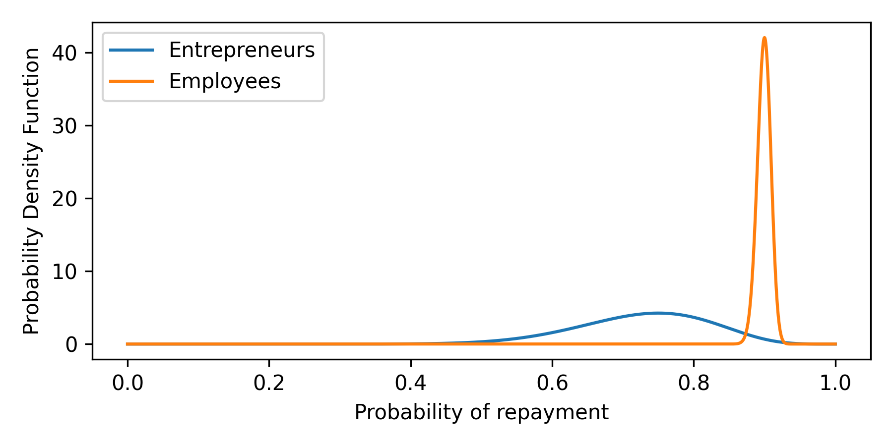
Notice how the posterior spans between 0.75 and 0.9 - these are the probabilities for two different input types, and indeed, accuracy cannot be lower or higher than this. Since there are more employees, the distribution is skewed towards 0.9, which is an employee's repayment probability. In reality, we are never sure whether these probabilities are perfectly calibrated - we always observe only some sample of the data, not the whole population. Let's say that before running the experiment, we saw 1000 employees, and 900 of them (90%) repaid the loan. We also saw 20 entrepreneurs - 15 repaid (75%). Are probabilities calibrated, then? They are on the sample, but we don't know if they are on the population. We can model the true probability distribution given predicted probability with Beta again. Here's how it looks for the described case:

Figure 2. Distribution of population probability of repaying the loan for the two types of applicants.

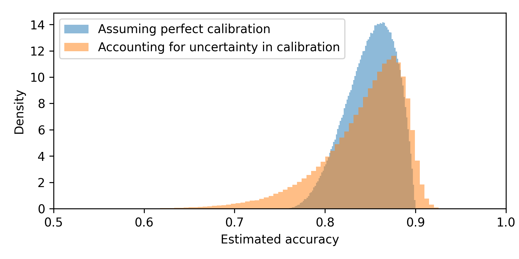
We again start the experiment and observe the same data as previously (5 applicants, with 1 being an entrepreneur). To get population-level accuracy distribution, we do the following: we sample from the applicant-being-entrepreneur probability distribution first (just like previously). Then, for the proportion sampled, we sample from posteriors of the true probabilities that the applicant will repay the loan given the applicant type and estimate accuracy for sampled numbers (using CBPE). Here is what we get compared to what we got previously (with perfect calibration assumption):

Figure 3. Posterior of estimated accuracy with perfect calibration (blue) and calibration measured on data (orange).

As expected - the new posterior is less precise (wider) as it accounts for more uncertainty. Notice how the left tail became heavier compared to the right tail. This is because we have more uncertainty for the calibration of entrepreneurs (the ones with a mean of 0.75 of repayment). The right tails became only slightly heavier - there's a lot of previous data on employees, and there's not much uncertainty around the calibration for this type of applicant.

The estimated performance (without labels) posteriors will often become wider for the same amount of data compared with realized performance (with labels) posteriors. That is because there is uncertainty around calibration that must be considered - there is no perfect calibration in the real world. Since, during the experiment, we don't gather any more data on the calibration (as there are no labels available), the uncertainty related to calibration does not diminish. This means that at some point, performance metric estimation does not get any more precise (HDI is not becoming narrower) even when we gather more data.

In real life, there are no models with single binary features only - there are multiple features, some of which are continuous. So, in the final solution, we cannot condition the feature value; we will condition it based on the predicted probability the model estimates. Instead of getting the posterior of population-level target probability distribution per feature value (like shown in Figure 2), we will calculate it per probability predicted by the model. There is another limitation here, though. We may have only one entry in the data for a specific value of predicted probability. Let's say that the model returned a probability of 0.7 only for one observation with a label, which was 1. Should we then condition on that predicted probability value and calculate the true target probability distribution? That is an almost uniform distribution. At the same time, the very same model might have thousands of observations with a predicted probability of 0.71, which shows very good calibration. It seems reasonable to assume that the calibration for 0.7, which is relatively very close, is also good. That is one of the reasons why we decided to bin observations into equal-sized buckets and condition those buckets in the actual solution. That also is beneficial for modeling the uncertainty around drawing data from the inputs. The actual implementation is described below.

The algorithm

The algorithm can be split into two parts: the fitting part on reference data and the inference part on experiment data. Based on the reference data, we determine the bins (based on predicted probability) and estimate the true label posterior distribution within each bin.

- $\hat{ypp}$ predicted probability - $\hat{y}$ - binary prediction - $y$ - label - $i$ - bin indicator.

ON REFERENCE DATA

1. Define bin edges:

   1. Split predicted probabilities $\bold{\hat{ypp}_{ref}}$ into n (default n=10) equal-sized bins.
   2. Add an extra bin edge equal to the prediction threshold (that is, the threshold above which the prediction is 1). This ensures that no bin contains mixed predictions of 1 and 0.

2. For each bin, based on observations inside the bin:

   1. Store prediction value (0 or 1).

   2. Create a target posterior distribution for each bin such that: $Beta(\alpha=sum(y=1)+1, \beta=sum(y=0)+1)$ and store it.

ON EXPERIMENT DATA:

3. Split data into bins using bin edges from step 1.

4. Get a posterior of binned $\hat{ypp}$ distribution:

   1. Count observations in each bin.

   2. Create a Dirichlet posterior distribution that tells the probability of observing each bin. The number of categories () is equal to the number of bins. The concentration parameter () for each category/bin is equal to the number of observations in that bin + prior. Prior is equal to the width of the bin. So all the priors sum up to 1. Such a prior means observing any bin is equally likely.

5. Calculate the mean $\hat{ypp}$ for each bin based on experiment data belonging to that bin. Denote it $\hat{ypp}_{exp, i}$.
6. Sample from the posterior of the estimated performance metric:

   1. Sample from Dirichlet distribution created in step 4. It tells the probability of observing each category (bin) given the experiment data seen so far.

   2. Sample from each bin's true label distribution posteriors (created in step 2.2).

   3. Estimate the performance metric value based on: true label distribution for each bin (step 6.2), the weight of each bin (step 6.1) the model mean predicted probability of each bin (step 5) or the model binary prediction for each bin (step 2.1). The mean predicted probability is needed when estimating ROC AUC. Other available metrics (accuracy, precision, recall, f1) use binary predictions.

7. Repeat 6 to get a large enough sample of the posterior of the estimated performance metric.

8. Fit Gaussian KDE to get a PDF of the posterior of the metric of interest.